Secondary Stress: Proteomics
Analysis of QE data
downloaded mzXML files for QE data onto Mac mini PC from the server where Jimmy uploaded them. The xml files were previously downloaded.
Enrichment analysis of differentially expressed proteins in QE data for ambient vs. high pCO2 only (MS samples included but not acknowledged as different treatment). Made a list of all of the unique SPIDs that correspond to the proteins that had at least 10 spectral hits across replicates - this is the background for DAVID. Made 4 gene lists for analysis: 1) SPIDs corresponding to proteins that were differentially expressed according to a t-test, 2) SPIDs of proteins that were at least 2-fold up-regulated, 3) proteins at least 2-fold down-regulated, 4) all 3 previous categories combined.
For category 1 (t-test), enriched GO terms were protein folding, peripheral nervous system development, mitotic cell cycle, macromolecular complex assembly, cell cycle process, macromolecular complex subunit organization, protein complex biogenesis.
For category 2 (up-reg at least 2 fold): protein heterooligomerization, regulation of transcription, regulation of transcription DNA-dependent, transcription, protein complex biogenesis, protein complex assembly, macromolecular complex subunit organization, regulation of RNA metabolic process, macromolecular complex assembly, pyrimidine nucleotide biosynthetic process, pyrimidine nucleotide metabolic process, regulation of transcription from RNA polymerase II promoter, positive regulation of nucleobase, nucleoside, nucleotide and nucleic acid metabolic process.
For category 3 (down-reg at least 2 fold): muscle organ development, cellular protein localization, muscle tissue development, skeletal muscle organ development, cellular macromolecular localization, intracellular protein transport, induction of apoptosis, protein import, regulation of transcription DNA-dependent.
For category 4: mitotic cell cycle checkpoint, protein complex assembly, protein complex biogenesis, regulation of transcription DNA-dependent, cell cycle checkpoint, macromolecular complex assembly, macromolecular complex subunit organization, pyrimidine nucleotide metabolic process, pyrimidine nucleotide biosynthetic process, membrane organization, response to abiotic stimulus, protein import, protein oligomerization, detection of stimulus, enzyme linked receptor protein signaling pathway, positive regulation of nitrogen compound metabolic process, positive regulation of transcription from RNA polymerase II promoter, sulfur amino acid metabolic process.
January 2, 2013
Secondary Stress: Proteomics
Analysis of QE data
From stats done 12/20/12, made list of unique protein IDs of differentially expressed proteins (for each treatment comparison the protein is either differentially expressed according to the t-test with p<0.05, or according to fold change of at least 2 up- or down-regulated). This is 1,086 proteins. Made a fasta file of the protein sequences (from genome v9) corresponding to these CGI IDs in Geneious.
Did DESeq on protein expression data from QExactive. Created 2 input files: one to compare effects of pCO2 (on non-mechanically stressed oysters only) and one to compare the effects of MS on the ambient pCO2 oysters. Both were treated as single-end libraries. The comparison of the pCO2 treated oysters yielded one protein that was differentially expressed with an adjusted p-value of < 0.1: CGI_10005508 (this protein is already included in the differentially expressed list described above). There was no protein expression different due to mechanical stress in the ambient pCO2 oysters according to DESeq.
protein CGI_10005508 is putatively carboxymethylenebutenolidase
December 21, 2012
Secondary Stress: Proteomics
Continuation of analysis of QE data
Joined file of proteins with at least 10 spec counts across replicates to GO and GO Slim terms in Galaxy. In Excel, separated the file into 3 parts based on GO terms: cellular components, molecular function, and biological processes. For today, will just do analysis at the biological processes level. For each of the 3 sub-files, filtered to maintain unique protein-GO term combinations. Kept only proteins that were annotated with SPIDs with an evalue of less than or equal to 1E-5. Did the same process for GO Slim terms.
To create file of spec counts per GO term, sorted spec counts, protein ID, and GO term by GO term. Removed redundant entries so that a protein is not counted multiple times for one GO term. For each GO term, summed the spec counts for each oyster and then pasted into a new spreadsheet. The new spreadsheet has GO terms in the first column followed by the sum of all spec counts for that term for each oyster. Did the same for GO Slim biological processes.
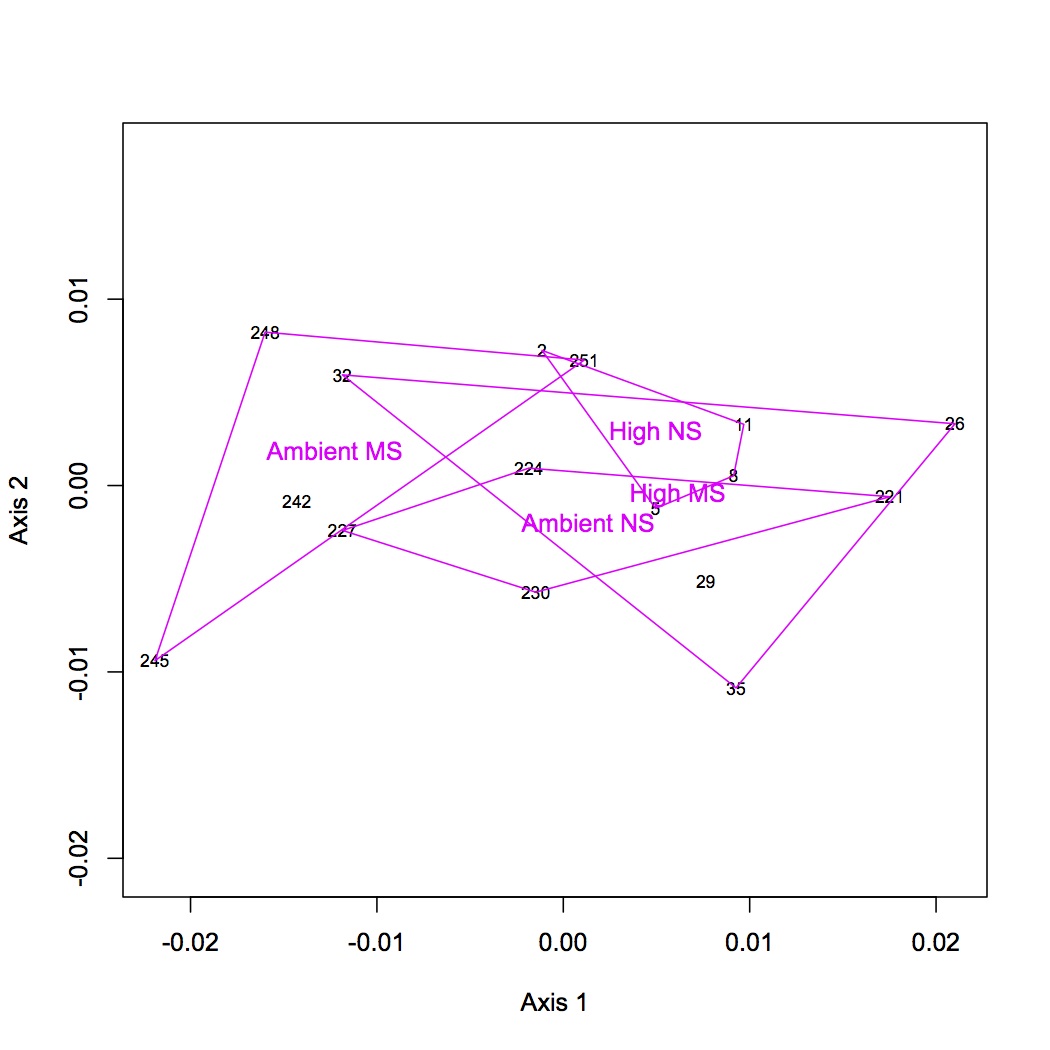
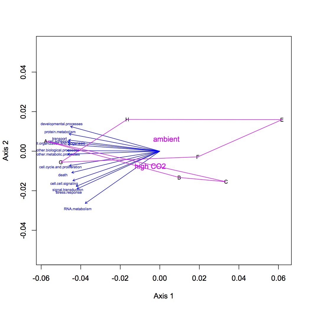
Did NMDS (described 12/20/12) on oysters described by GO or GO Slim terms and ANOSIM looking at effect of pCO2, MS, and combination of MS + pCO2. There was no difference in expression among treatments at the GO or GO Slim levels.
NMDS using GO terms:
http://eagle.fish.washington.edu/oyster/NMDS%20GO%20processes%20loadings%20122112.jpg
http://eagle.fish.washington.edu/oyster/NMDS%20GO%20processes%20polygons%20122112.jpg
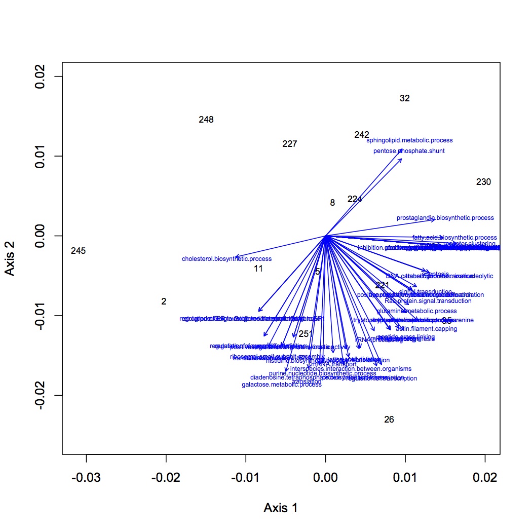

NMDS using GO Slim:
http://eagle.fish.washington.edu/oyster/NMDS%20GO%20slim%20processes%20loadings%20122112.jpg
http://eagle.fish.washington.edu/oyster/NMDS%20GO%20slim%20processes%20polygons%20122112.jpg

December 20, 2012
Secondary Stress: Proteomics
Analysis of proteomic data from the QExactive
In Galaxy, viewed joined file and selected "view all". Copied and pasted into text wrangler. Under Search > Find searched for "QE" and replaced with "\r" enabling grep. This makes a line break at every QE. Saved and opened in excel to edit (some columns need re-aligning).
Removed proteins that had fewer than 10 spectral counts across all replicates (remaining proteins = 2,437). Summed spectral counts across technical reps, within biological reps.
Annotated the proteins joined to the summed spec counts in Galaxy.
Statistics in Excel to get an idea of potential important proteins in differential expression. For the following treatment comparisons, calculated p-value (type 2, 2-tailed t-test) and fold change (stressor/control): mechanical stress in High pCO2, MS in ambient pCO2, MS, pCO2.
t-test results: 135 proteins were differentially expressed due to MS at high pCO2, 97 were differentially expressed due to MS at ambient pCO2, 119 were differentially expressed due to MS across pCO2 treatments, 145 were differentially expressed due to pCO2 (this included oysters that had been exposed to MS).
fold change results (down regulated at least 2 fold): 267 due to MS at high pCO2, 322 due to MS at ambient pCO2, 177 due to MS across pCO2, 206 due to high pCO2.
fold change results (up regulated at least 2 fold): 236 due to MS at high pCO2, 164 due to MS at ambient pCO2, 155 due to MS across pCO2, 129 due to high pCO2.
Made 4 datasets from proteomic data for NMDS and ANOSIM: 1 dataset had all the proteins included, the second dropped low abundance proteins (expressed in < 1/2 oysters), the third dropped high abundance proteins (occurred in >95% of the oysters), and the fourth dropped both low and high abundance. Did NMDS using a Bray-Curtis dissimilarity matrix and ANOSIM. There was no significant difference among treatments at the protein level. Below are NMDS for the dataset with all proteins (including low and high abundance). The loadings (blue arrows) are all proteins that contribute significantly to the distribution of objects (oysters) with a significance of p=0.01 or lower.
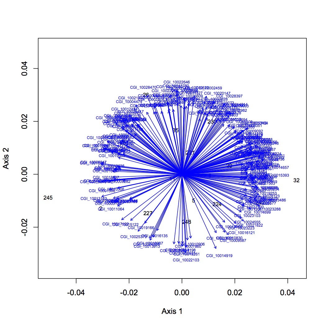
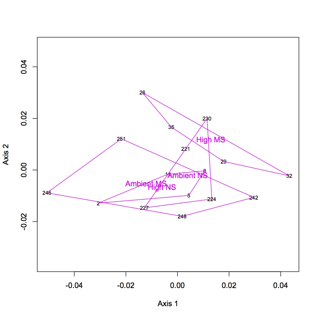
Tomorrow: NMDS and ANOSIM at GO and GO Slim level.
December 19, 2012
Secondary Stress: Proteomics
Joined all QExactive replicates to the QE sequenced proteome in Galaxy (replicates are joined in alpha numeric order, starting with 101B_2_01 and ending with 103B_251_03). Galaxy will not let me download the file right now so I'll try again tomorrow :(
December 18, 2012
Secondary Stress: Proteomics
Prepared QExactive protein prophet files for upload and joining in Galaxy.
Created a non-redundant list of all the proteins (with Protein prophet probability cutoff of 0.9) that were sequenced on the QExactive ("QE sequenced proteome"). There are 4265 proteins in the list.
December 14, 2012
Secondary Stress: RNA-Seq
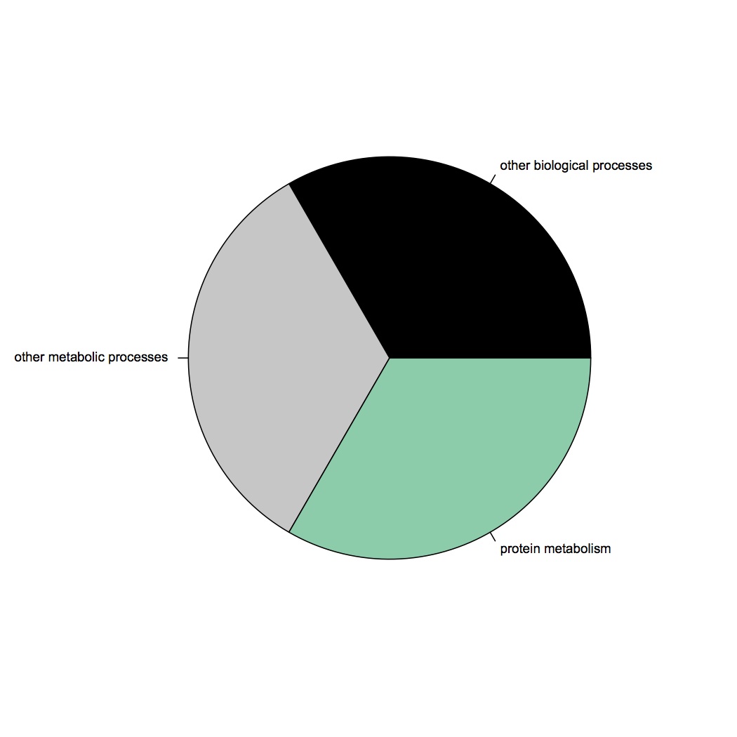
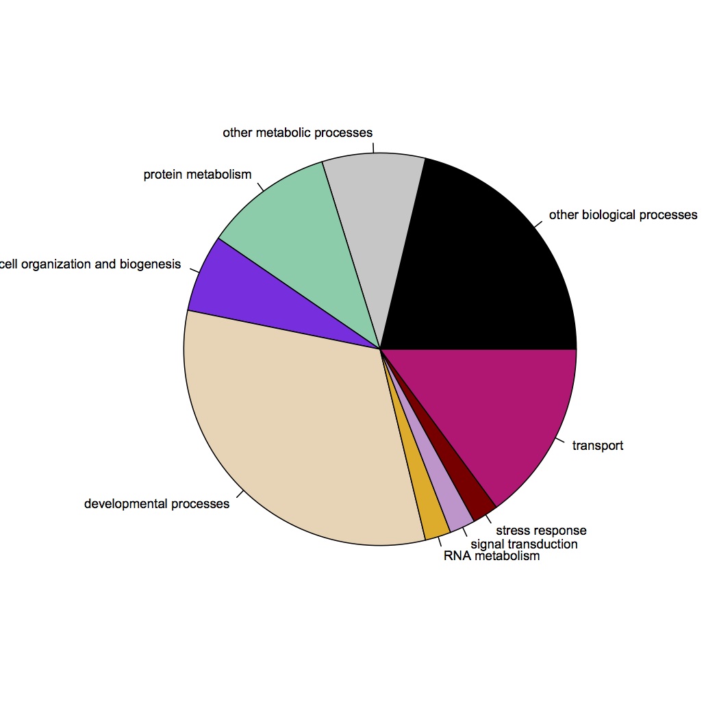
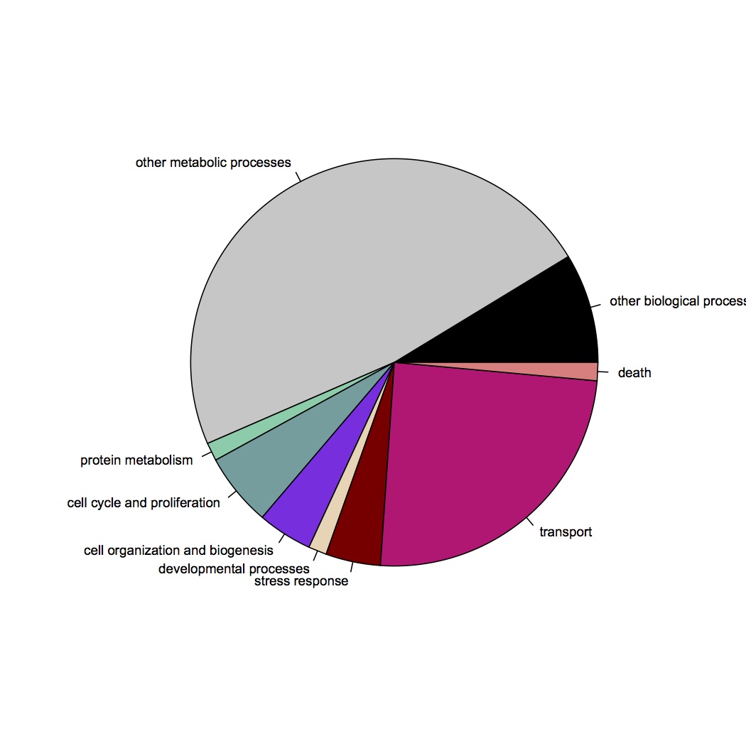
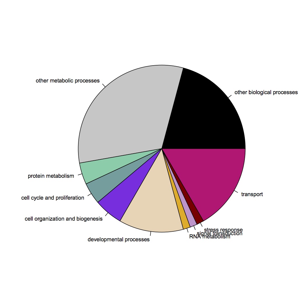
Ran DAVID analysis today for files prepared 12/13/12. For genes that were differentially expressed according to a t-test, there was an enrichment of GO terms for protein amino acid phosphorylation, sensory perception of light stimulus, visual perception, heparan sulfate proteoglycan biosynthetic process, heparan sulfate proteoglycan metabolic process, protein catabolic process. There were 60 GO terms enriched in the genes that were at least 2-fold more highly expressed at high pCO2. 40 GO categories were enriched in the genes up-regulated at ambient pCO2. For the group of genes differentially regulated (combination of the previous 2 groups), 63 GO categories were enriched. Below are pie charts of the GO Slim terms representing number of enriched GO terms for each category.
GO Slim categories corresponding to contigs differentially expressed according to t-test: http://eagle.fish.washington.edu/oyster/t.test%20sig%20diff%20GO%20Slim%20121412.jpg
GO Slim categories of contigs up-regulated at ambient pCO2 (at least 2-fold): http://eagle.fish.washington.edu/oyster/ambient%20pCO2%20upreg%20GO%20slim%20121412.jpg
GO Slim categories of contigs up-regulated at high pCO2 (at least 2-fold): http://eagle.fish.washington.edu/oyster/high%20pCO2%20upreg%20GO%20Slim%20121412.jpg
GO Slim categories of contigs differentially regulated at least 2-fold: http://eagle.fish.washington.edu/oyster/diff%20reg%20GO%20Slim%20121412.jpg
NMDS and ANOSIM at contig, GO, and GO slim levels excluding oyster D. No better resolution was achieved, ANOSIM for GO and GO Slim levels was insignificant.
NMDS of contigs without oyster D: http://eagle.fish.washington.edu/oyster/NMDS%20contigs%20no%20oyster%20D%20121412.jpg

NMDS of GO terms without oyster D: http://eagle.fish.washington.edu/oyster/NMDS%20GO%20no%20oyster%20D%20121412.jpg
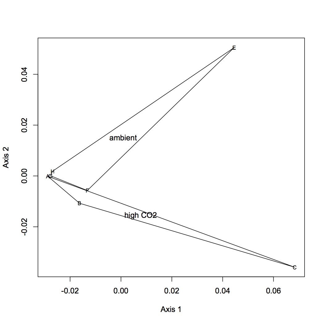
NMDS of GO slim without oyster D: http://eagle.fish.washington.edu/oyster/NMDS%20GO%20slim%20no%20oyster%20D%20121412.jpg
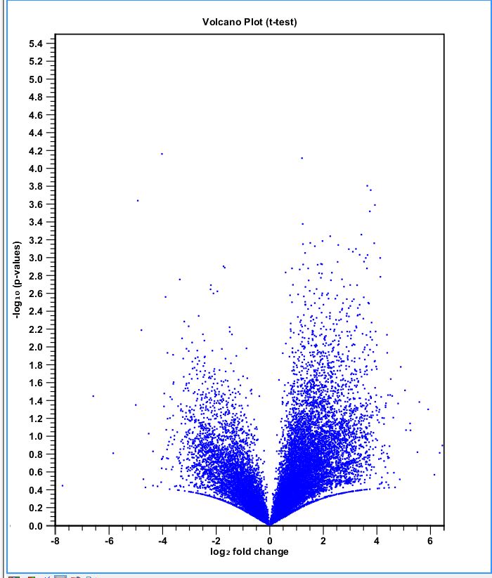
performed hierarchical clustering in CLC on expression experiment 121312. Used Euclidean distance, average linkage, original expression values. Also did statistical analysis on Gaussian data: T-test variances homogeneous (variances assumed to be equal), comparisons = all pairs, use original expression values, add corrected p-values for bonferroni and FDR.
volcano plot: http://eagle.fish.washington.edu/oyster/volcano%20plot%20121412.jpg
December 13, 2012
Secondary Stress: RNA-Seq
On 12/3/12 I did a de novo assembly of the 8 tag-seq libraries to make consensus isotigs. Also on 12/3 I did RNA-Seq of the libraries against this de novo assembly to get expression values for each isotig (the contig numbers are conserved across the de novo assembly and the RNA-Seq). On 12/4, all the RNA-Seq files were joined together to form the file "all isotig RNA-Seq joined". On 12/5, blasted the isotigs against Sigenae v8 for annotation.
Edited the file from 12/5 so that instead of isotig names reading "Consensus from Contig 116" they read "Contig116". This file gives the number of reads mapped to each isotig by sample library (8 libraries). The only isotigs used in further analysis are those with at least 10 reads mapped across the 8 libraries. Saved tab-delim text file as "library reads mapped to isotigs".
In Galaxy, joined isotig reads mapped file with isotig blastn sigenae v8 results. Then joined with Cg Sigenae8 best hit to get SPID annotations. Then joined with Cg Sigenae ontology to annotate with GO terms. Also joined with Go Slim terms. File is called "isotig reads mapped annotated".
To get number of reads per isotig, made 8 separate pivot tables (1 for each library) of the sum of number of mapped reads per Sigenae accession number. For each library, a large number of reads map to isotigs that do not have a blastn result against the Sigenae database.
Made input file for DESeq of total reads mapped per contig in each library (file = Sigenae reads DESeq).
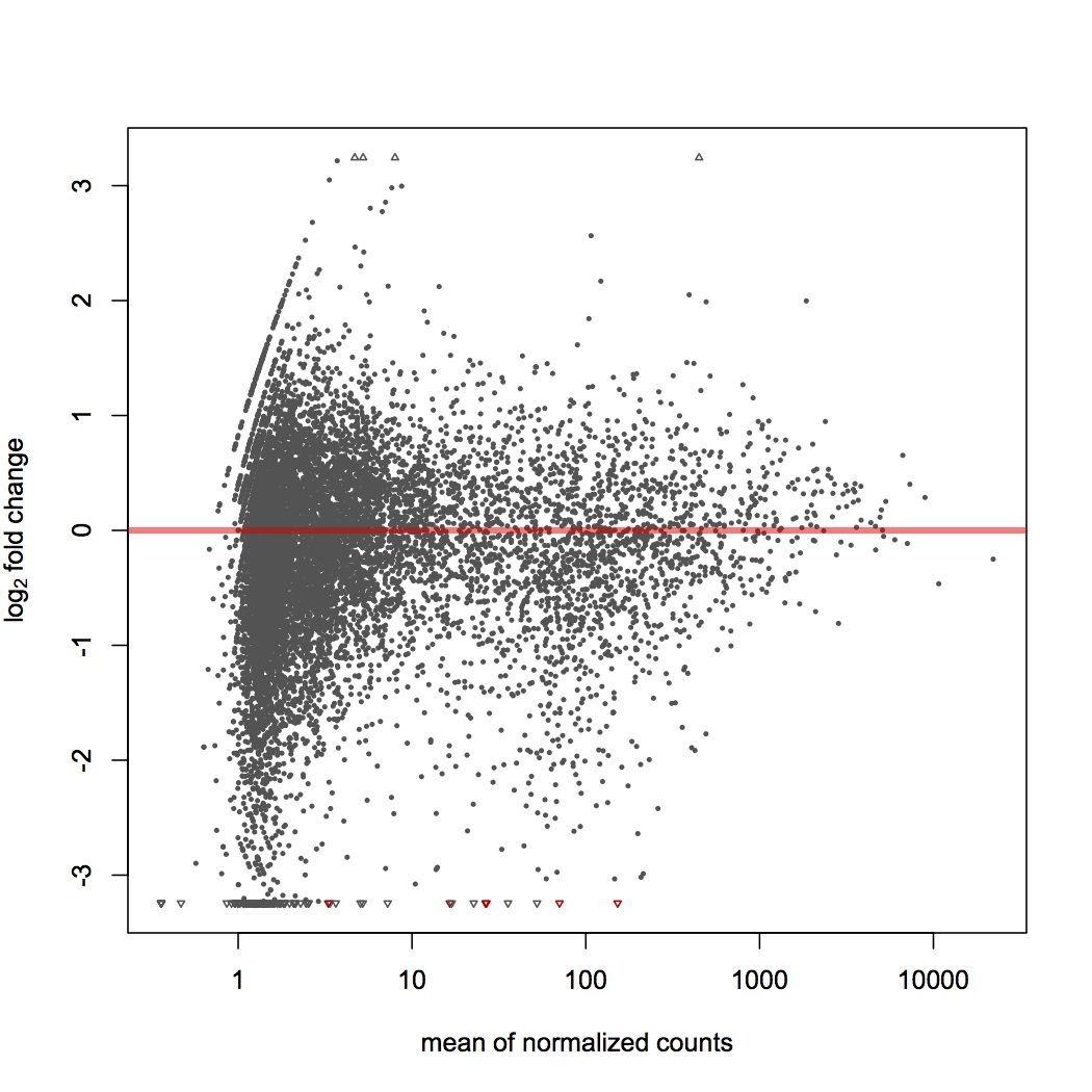
DESeq plots:
variance estimation: http://eagle.fish.washington.edu/oyster/variance%20estimation%20sigenae%20121312.pdf
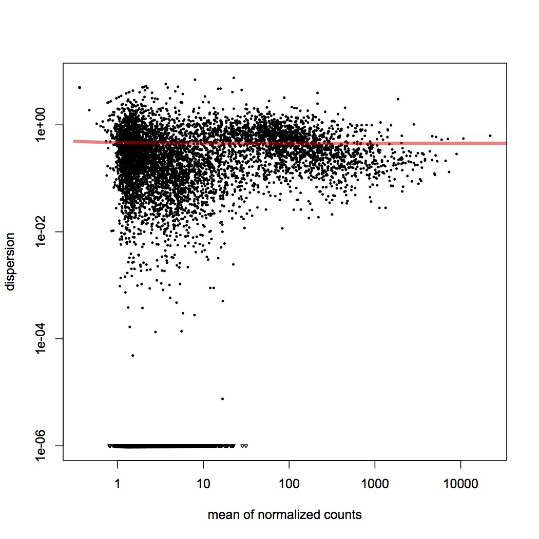
differential expression: http://eagle.fish.washington.edu/oyster/diff%20exp%20sigenae%20121312.pdf
pvalues: http://eagle.fish.washington.edu/oyster/pvalues%20sigenae%20121312.pdf
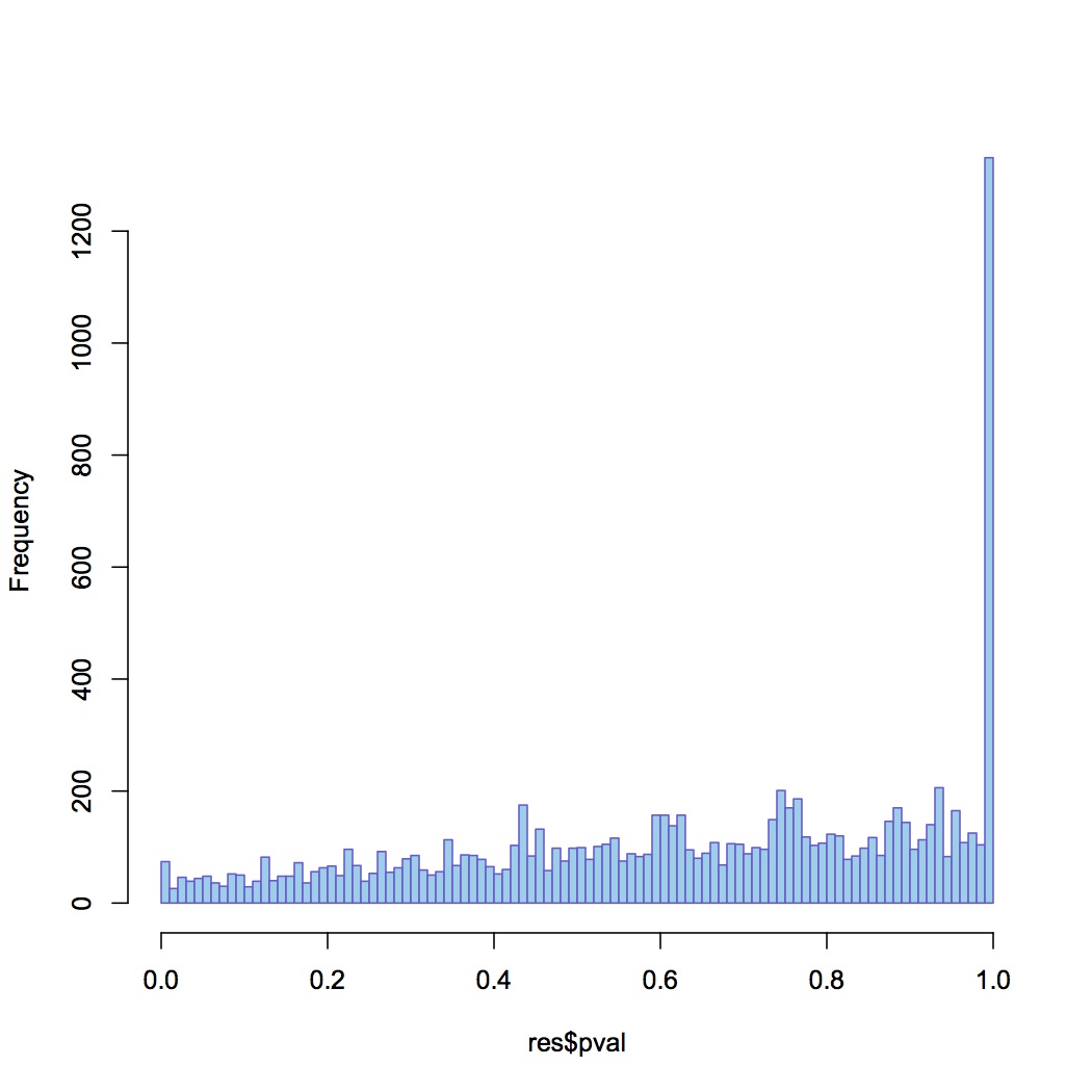
6 genes are differentially expressed (adjusted p-value < 0.05), all are up-regulated in the high pCO2:
CU682172 = hyaluronan-mediated motility receptor
FV2TRRU02GXXJN = heat shock 70 kDa protein
AM857082 = TPR and ankyrin repeat-containing protein
CU999485 = DNA binding protein SMUBP
CU996918 = D. rerio hypothetical protein
FU6OSJA01A8KLU = not annotated
Exploration of differentially expressed genes as determined by t-test. Did a t-test (type 2, 2-tailed) in Excel for each Sigenae contig based on sum of all reads. Annotated the contigs with SPIDs. Also divided the sum of the reads for the high pCO2 libraries by the sum of the reads for the ambient pCO2 library for each Sigenae contig. Now there are 2 new metrics for looking for differentially expressed genes: significance from the t-test (p<0.05) and fold change. To look for enrichment of GO categories in these groups of genes, made a DAVID input file with genes that are sig diff according to the t-test, highly expressed (2-fold or greater) in high pCO2, highly expressed in ambient pCO2. Removed redundancy from spid lists. The background for DAVID is the SPIDs annotating all of the Sigenae contigs (all SPID annotations have an evalue of less than 1E-5).
DAVID is currently down so may need to run these analyses tomorrow.
Some of the genes that are differentially expressed according to the t-test (335 total) are hsc70, hsp70, cytochrome p450, v-type proton ATPase, ficolin.
A total of 2121 genes were expressed less at high pCO2 compared to low pCO2 (by at least 2-fold). These included cathepsin, hsp70, ficolin, v-type proton ATPase, caspase-14, metallothionein, cytochrome p450, hsc70, defensin.
885 genes were expressed at least 2-fold more highly in the high pCO2 treatment, including multidrug resistance-associated protein, hsp70, glutathione peroxidase, v-type proton ATPase, peroxiredoxin 6.
RNA-Seq experiment on CLC. Set up experiment with the RNA-Seq files from 12/3/12 (reads mapped back to de novo assembly of isotigs). Parameters: two-group comparison unpaired, use existing expression values from samples. Assigned libraries to groups "high pCO2" and "ambient". Saved in folder "expression experiment 121312".
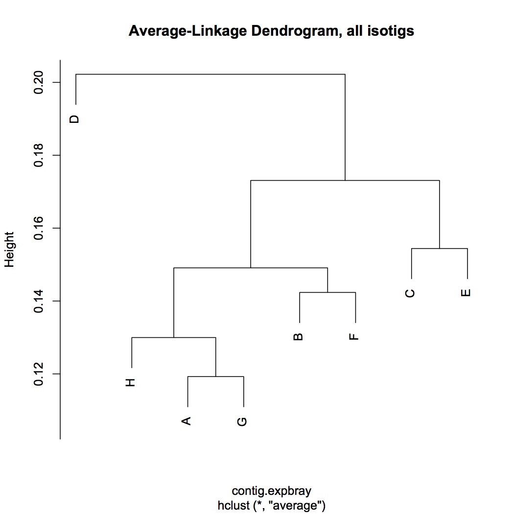
Multivariate analysis of RNA-Seq data, starting with contig level. Input file is sum of reads across isotigs for each contig. Did parallel analyses for the entire data set (10341 contigs) and for the dataset without low abundance genes (expressed in fewer than 8 oysters, 4228 contigs). Did log(x+1) transformation and used bray-curtis dissimilarity coefficient. Did hierarchical agglomerative clustering and made average linkage dendrograms. There was no clear pattern according to treatment.
all contigs: http://eagle.fish.washington.edu/oyster/average-linkage%20dend,%20all%20isotigs%20121312.pdf
without low abundance contigs: http://eagle.fish.washington.edu/oyster/avg-linkage%20dend,%20no%20low%20abundance%20isotigs%20121312.pdf
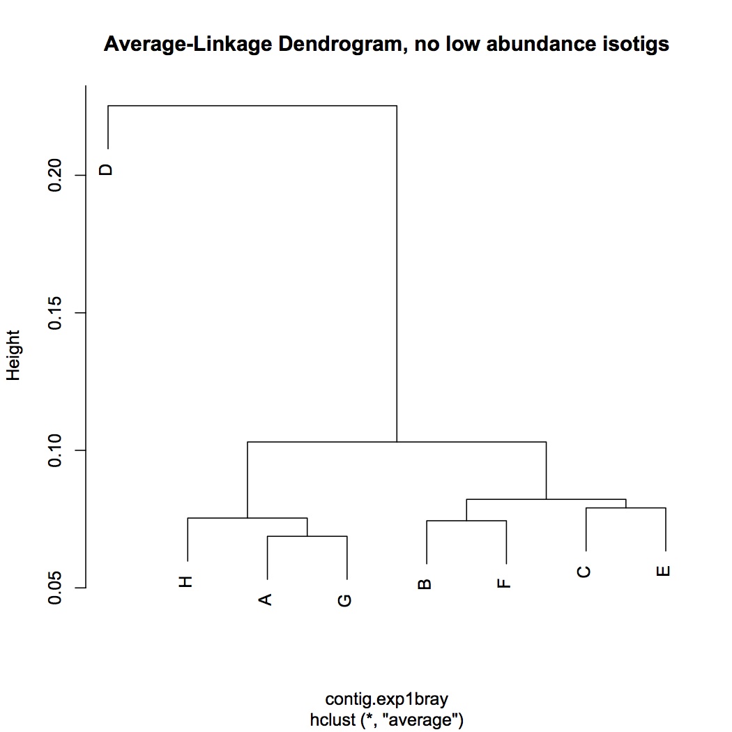
Also did clustering with euclidean distance instead of bray-curtis and dendrograms looked identical using the different coefficient.
Next did NMDS. NMDS plots do not show vector loadings because there were too many arrows.
NMDS all contigs: http://eagle.fish.washington.edu/oyster/NMDS%20all%20isotigs%20121312.pdf
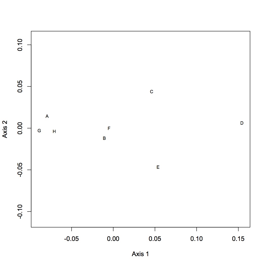
NMDS no low abundance: http://eagle.fish.washington.edu/oyster/NMDS%20no%20low%20abundance%20isotigs%20121312.pdf
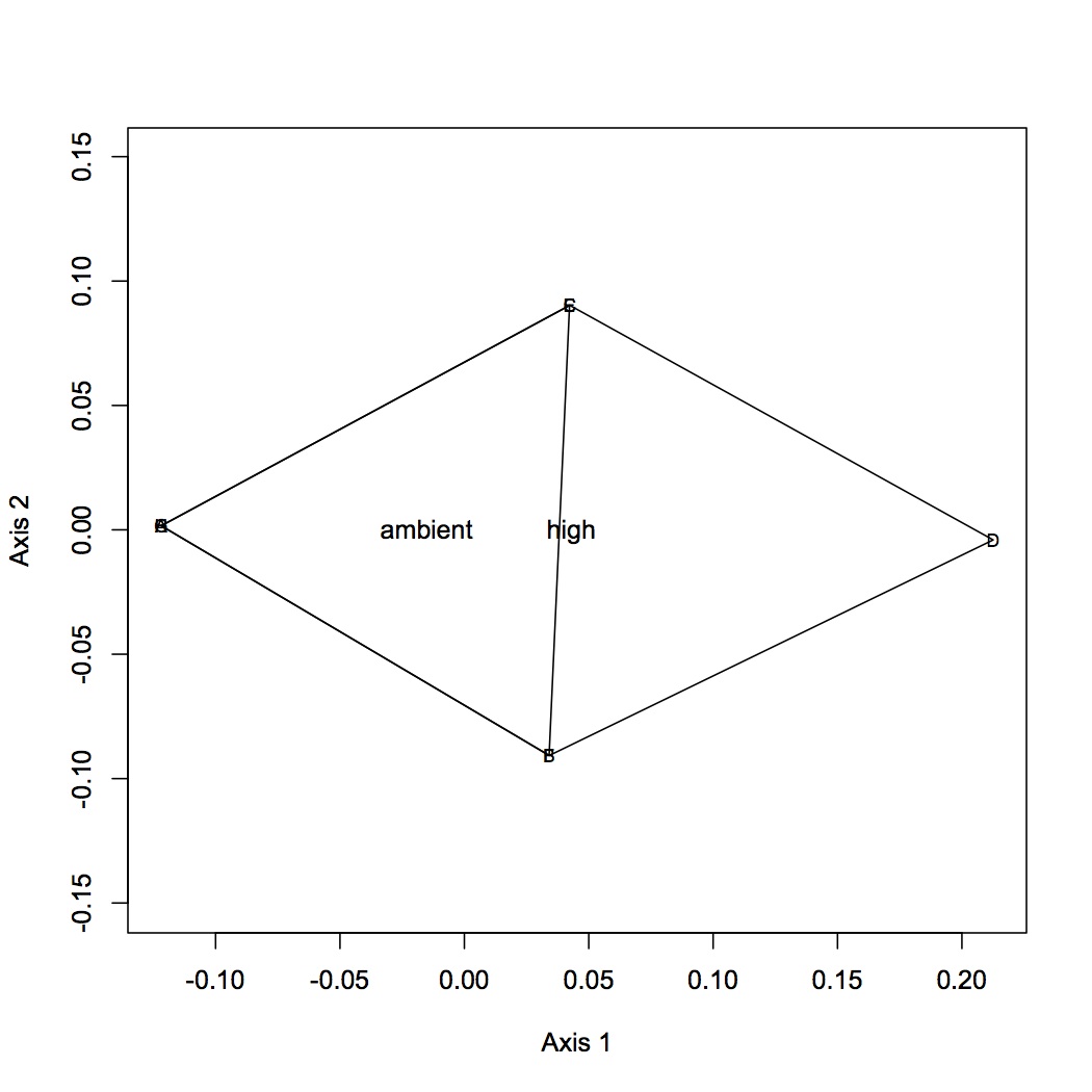
There was no significant effect of treatment on gene expression for either dataset using ANOSIM.
Multivariate analysis at GO and GO Slim levels (instead of individual contig). Annotated contigs in Galaxy with GO and GO Slim terms. For now I will only work with the biological processes terms. Made worksheets of contigs, read counts for each library, and GO or GO slim terms (removed redundancies). Made pivot tables for each library: sum of reads within GO or GO slim category.
NMDS at go and go slim level still shows lack of resolution between treatment groups. This may be because oyster D is an outlier. Will try same analysis but without oyster D.
December 12, 2012
Secondary Stress: Proteomics
Continuation of Skyline analysis.
Brendan (developer of Skyline) responded to my query regarding how to treat the different precursor charges:
It really depends on what you are doing. If you measured both charge states and the data is good, then you would probably get a more accurate measurement of peptide abundance by summing the TotalArea values of both, under the principle that more ions measured will increase your precision.
If one charge state is a very small fraction of another, and has a totally different lower limit of quantification (LOQ), then, yes, you will probably want only the better precursor, since including the worse performing precursor is likely just decrease your linear range of detection, if you sum the two, and using them separately will just give you two different measures for the same thing, with one being provably worse than the other
It seems that the precursor charge 2 is less than half of the 3 charge state. Peptides that have only one charge state are a 2. Based on this, I'm just going to keep the data for the 2 charge state and discard the 3 state for further analyses.
For high pCO2 and high pCO2 + MS, created input files for Galaxy of the Prot-Pep combined indicator and the average peak area for that peptide. Made a backbone to join these files to of the prot-pep names for each treatment. Annotated proteins with SPIDs.
Created column in spreadsheet (MS vs NS) of the avg total peak area for the high pCO2 MS samples divided by the avg total peak area for high pCO2 (NS) samples. Some of the peptides that were up-regulated in the mechanically stressed oysters are beta-hexosaminidase (MS/NS = 206.031453), calmodulin (MS/NS = 103), clathrin (MS/NS = 18), putative universal stress protein (MS/NS = 8), myosin (MS/NS = 6), dual oxidase (MS/NS = 3), Some of the peptides that were down-regulated in the MS oysters included dual oxidase (MS/NS = 0.006), MAPK (MS/NS = 0.17), HSP70 (MS/NS = 0.2), stress-induced phosphoprotein (MS/NS = 0.38), v-type proton ATPase (MS/NS = 0.4), cathepsin L (MS/NS = 0.44). Next step for these proteins is to do an enrichment analysis for the up- and down-regulated proteins in mechanical stress. Differential regulation = at least 2-fold difference in expression. Overall, 162 peptides were down-regulated with mechanical stress at high pCO2 and 48 were up-regulated.
Repeated the same steps in Skyline to compare expression profiles between the high and ambient pCO2 oysters (no MS) and the ambient MS oysters vs. controls.
In ambient versus high pCO2, 71 proteins were upregulated at high pCO2, including dual oxidase (high/ambient = 212), MAPK (high/amb = 5), clathrin (high/amb = 3.7), HSP70 (high/amb = 2.8), v-type proton ATPase (high/amb = 2.5). 74 proteins were down-regulated, including glucose-6-phosphate isomerase (high/amb = 0.16), long chain fatty acid ligase (high /amb = 0.41).
In the comparison between ambient pCO2 no additional stress (NS) and mechanical stress (MS), 52 peptides were up-regulated in the MS and 246 were down-regulated.
Used all SPID annotations matching to proteins used in the analysis for the DAVID background. Generated lists of SPIDs corresponding to peptides down- and up-regulated at high pCO2 compared to ambient, ambient + MS compared to ambient, and high pCO2 + MS compared to high pCO2. All of the lists were filtered for redundancy. Enriched Gene Ontology categories are listed below for each treatment group (GOTERM_BP_FAT).
upregulated in Ambient MS: carbohydrate catabolic process, alcohol catabolic process
downregulated in High pCO2: cell adhesion, biological adhesion, blood vessel morphogenesis, vasculature development, blood vessel development
upregulated in High pCO2 MS: cognition, ion homeostasis, regulation of membrane potential, cellular ion homeostasis, cellular chemical homeostasis, chemical homeostasis, neurological system process, behavior
December 11, 2012
Secondary Stress: Proteomics
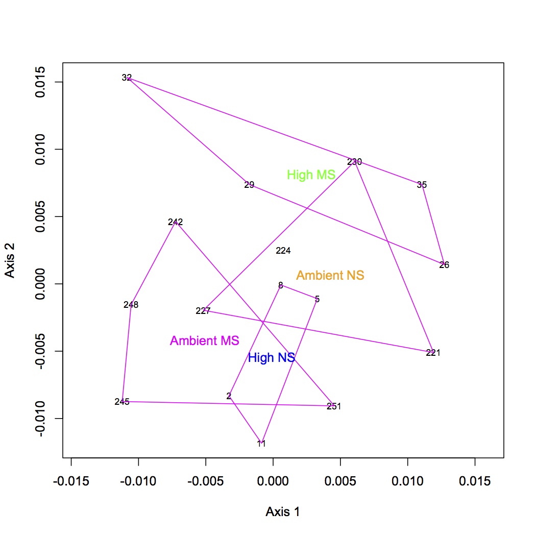
NMDS and ANOSIM of proteomics GO terms for molecular function. 170 unique GO terms were used in the analysis. There was no difference among treatments based on ANOSIM.
NMDS with GO molecular function loadings: https://www.evernote.com/shard/s242/sh/82b3879f-f671-44a5-9b31-1fceee9b4a56/0420e49a47260565269e13343a7a4b81
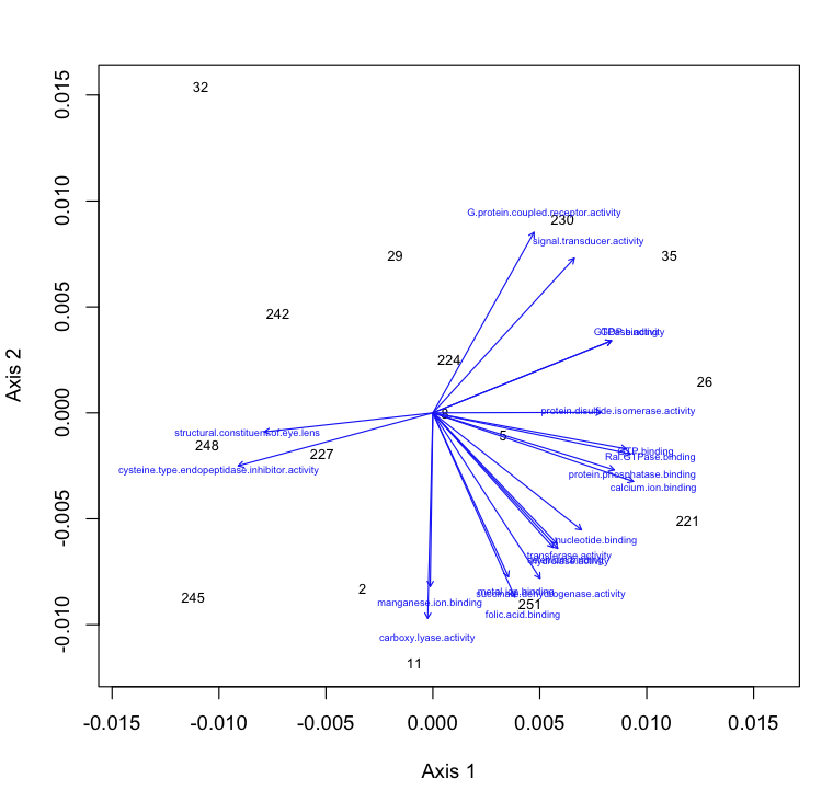
http://eagle.fish.washington.edu/oyster/GO%20function%20NMDS%20with%20loadings.pdf
NMDS with GO molecular function polygons:
https://www.evernote.com/shard/s242/sh/215f7268-5a83-48f5-91ce-62e765ce76ec/58b3abc34a9df224d24d68cebf2c0ca1
http://eagle.fish.washington.edu/oyster/GO%20function%20NMDS%20with%20polygons.pdf
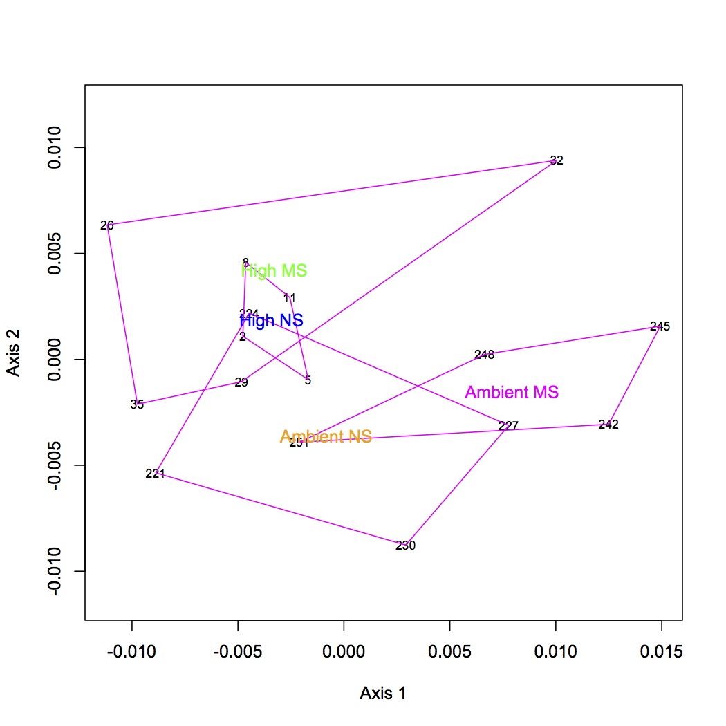
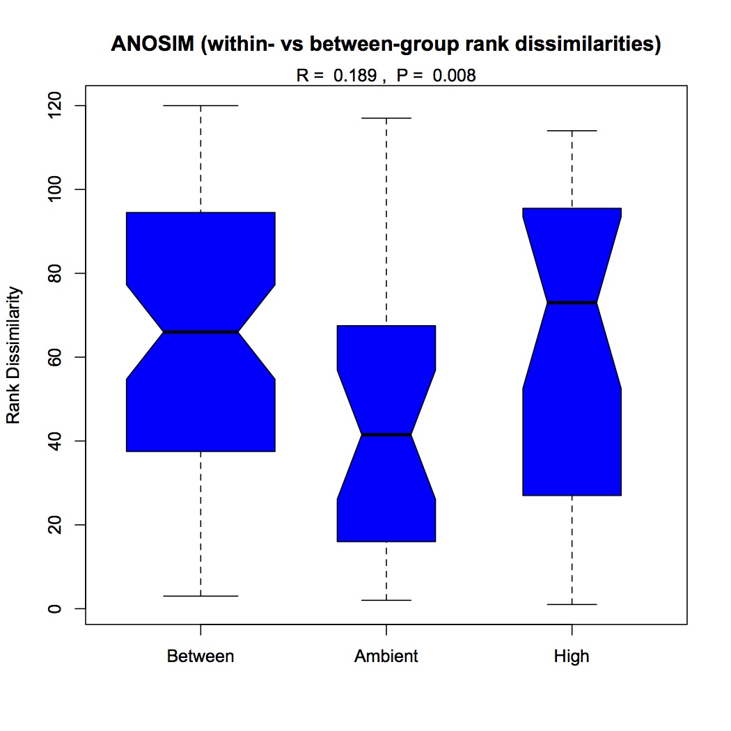
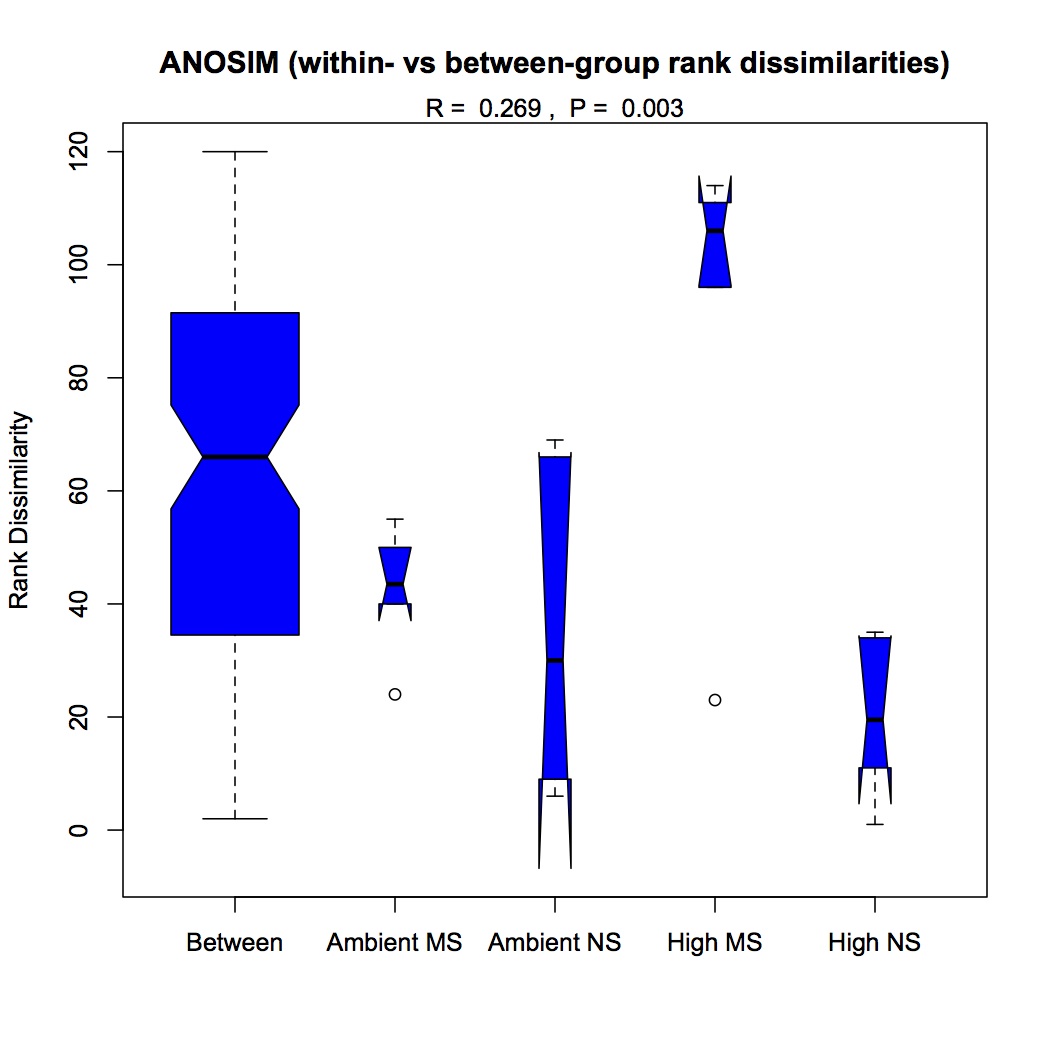
Repeated the same process except using GO Slim categories instead of GO. Divided up the cellular component, molecular function, and biological processes GO Slim terms. Removed proteins that were annotated with an evalue >1E-5. Removed redundant protein-GO Slim combinations. For now, I am only going to do the NMDS and ANOSIM for the biological processes GO Slim terms. Created an input file for R (as described 12/10/12). The ANOSIM analysis was significant for the effect of pCO2 on protein expression and the combined effects of pCO2 and MS, but not for MS alone.
NMDS GO Slim biological processes with loadings (p=0.01): https://www.evernote.com/shard/s242/sh/c32fd0f4-b716-4256-86f5-b48da431f038/cadfaa41f2874a1b924993636f1bd546
http://eagle.fish.washington.edu/oyster/GO%20Slim%20processes%20NMDS%20with%20loadings.pdf
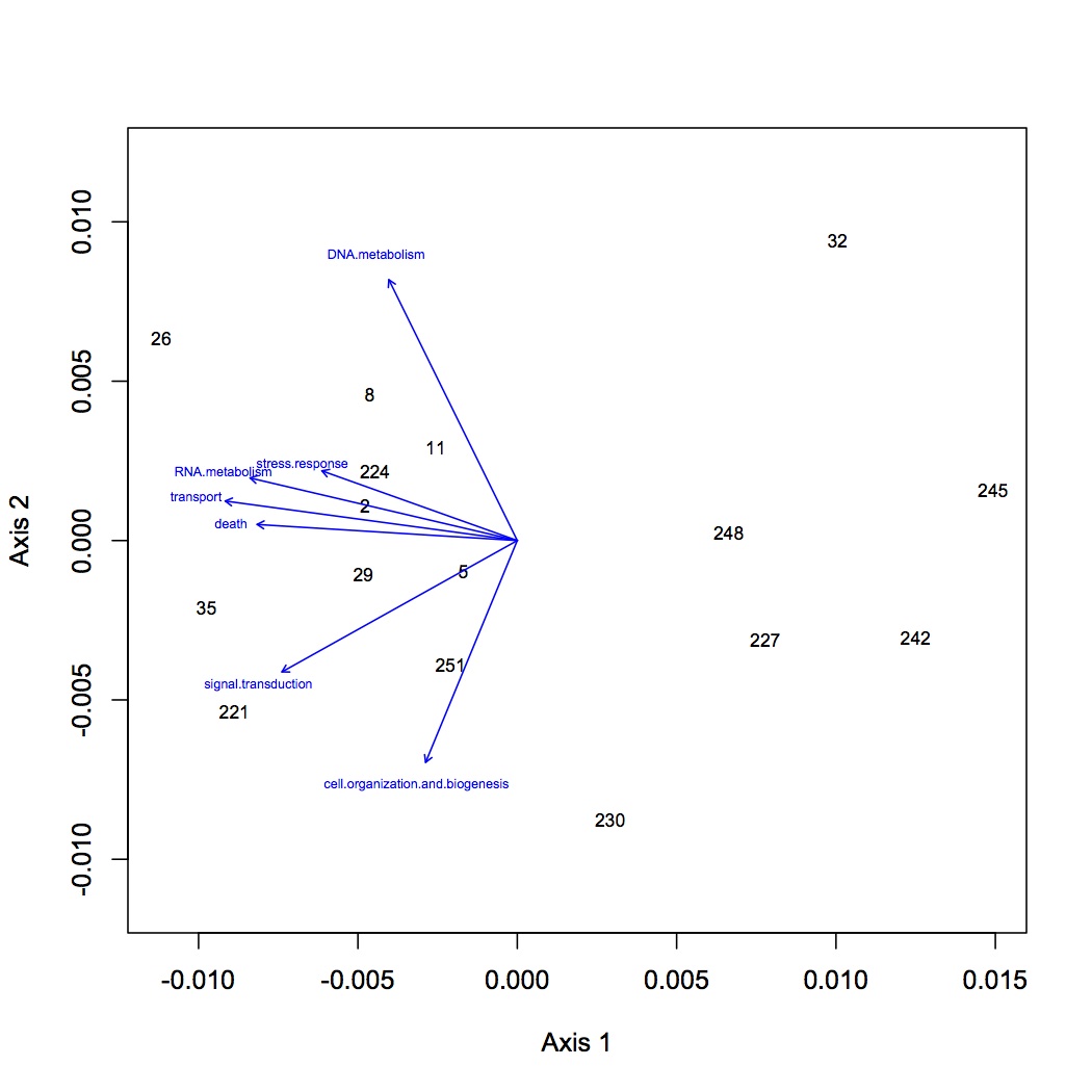
NMDS GO Slim biological processes with polygons: https://www.evernote.com/shard/s242/sh/a1faca45-9cb3-482b-bd9c-b007e50af15f/60d0a00efae2198edc34a543b7004455
http://eagle.fish.washington.edu/oyster/GO%20Slim%20processes%20NMDS%20with%20polygons.pdf
ANOSIM pCO2: https://www.evernote.com/shard/s242/sh/c800d8a4-76fb-4087-abd0-1dc4f99fb6e8/4373a8246c850818594c338d5a13a831
http://eagle.fish.washington.edu/oyster/GO%20Slim%20processes%20ANOSIM%20pCO2.pdf
ANOSIM pCO2 and MS: https://www.evernote.com/shard/s242/sh/3eb00b58-3d9f-44a5-aec1-5e5a257c6eb7/10028d4fcc08a96a146d696915a752a4
http://eagle.fish.washington.edu/oyster/GO%20Slim%20processes%20ANOSIM%20pCO2%20and%20MS.pdf
Enrichment analysis of proteomics data. Proteins used have at least 10 spectral counts across all replicates. The common list of proteins that fit this criterion are used as the backbone in DAVID. Made input file with one column of CGI protein accession numbers for each treatment group. Within each group, a protein is included in the input file if it has at least 4 spectral counts across the 4 oysters. The CGI accession numbers were joined with the blastx output (SPIDs) in Galaxy to make files for DAVID. Only unique SPIDs within treatment groups were kept in the final file for DAVID (v. 6.7).
The only GO term that was enriched (GOTERM_BP_FAT) was for high pCO2 + MS (regulation of transcription).
Analysis of proteins of interest in Skyline.
Downloaded zipped files (from Jimmy, mzXML_OT1, pepxml_OT1, pepxml_QE) from proteomics server onto "Mac" mini. These files extract to the files needed to build libraries in Skyline.
Also put protein of interest fasta file (see 12/6/12) onto Eagle to download and use in Skyline.
Settings > Peptide settings> Enzyme: Trypsin [KR|P]
max missed cleavages = 2
background proteome = none
Peptide settings > modifications > edit structural modifications: choose oxidation (M) from the drop-down list, check variable box.
Peptide settings > library > build: name = oyster proteins, keep redundant library, cut-off score = 0.95, lab authority = roberts.fish.washington.edu. Selected all "v9" interact files (these are the files that were searched against the genome and have been filtered for more probable proteins). pick peptides matching library.
Settings > transition settings > Filter: precursor charges = 2,3,4; ion charges = 1,2,3; ion types =p; auto-select all matching transitions.
transition settings > library: uncheck if a library spectrum is available, pick its most intense ions
transition settings > full-scan: isotope peaks included = count; precursor mass analyzer = orbitrap; peaks = 3, resolving power = 60,000 at 400, use only scans within 5 minutes of MS/MS IDs.
File > import > FASTA to import proteins of interest determined by prior analysis (C. gigas proteins for Skyline.fasta).
Settings: Integrate all
View > peak areas: replicate comparison
View > peak areas: right click and normalize to > none
All raw data files were imported as single injections.
Created export format for report titled "Oyster report". All 4 treatments are exported as separate csv files (in folder Skyline output 121012). In Excel, created worksheet of protein name, peptide sequence, sample name, total area, and cvtotalarea. Removed redundant entries. Created new column next to total area called prot-pep and concatenated the protein name and peptide sequence. Then selected the prot-pep and totalarea columns and made a pivot table with the prot-pep name as the row labels and the total area as the sum values (make sure to select sum!). This gives a table with the total sum of the peptide peak areas for each peptide (i.e. expression). Made another pivot table except with the average of the total area for each peptide.
There were redundancies in the original output file (some of the peptides had multiple peak areas for a sample), so re-exported the file with the columns: precursors charge, precursors isotope label type, precursors modified sequence. New file is called Skyline high pCO2 additions.csv. Also exported results for high pCO2 with mechanical stress.
The redundancy is caused by different precursor charges (2 vs 3). I'm not sure how to deal with this yet...
December 10, 2012
Secondary Stress: Proteomics
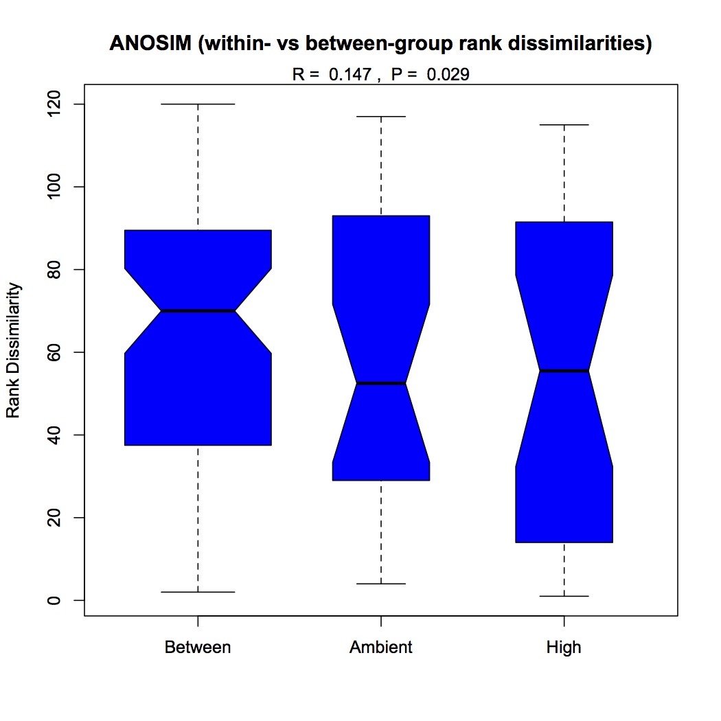
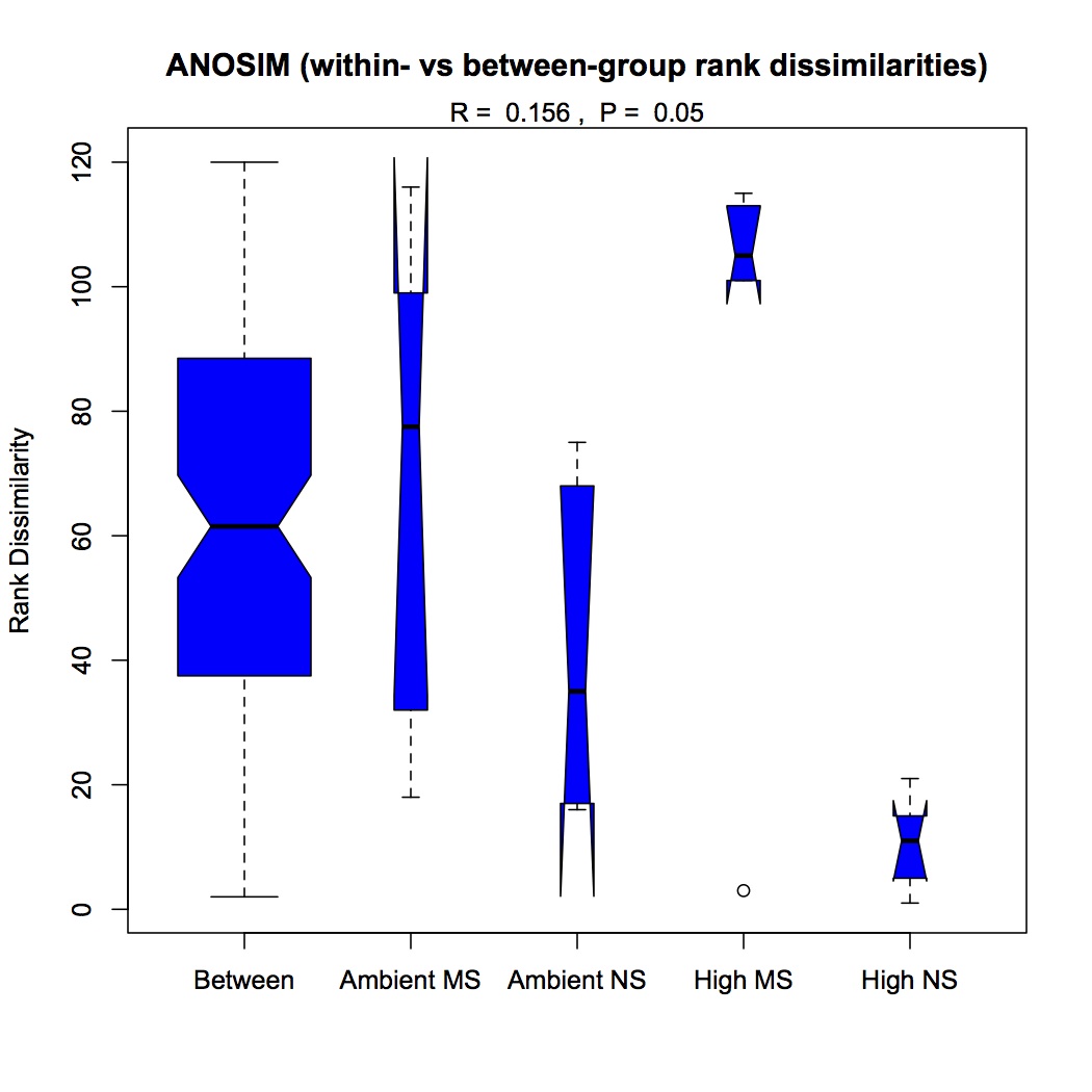
Did ANOSIM on protein expression visualized in NMDS 12/7/12. Created csv file with 3 columns describing the 16 oysters (oyster names in first column). One column had just the pCO2 treatment designators, one column had just MS, and one had the combination of the 2 stresses. ANOSIM was performed 3 separate times using the 3 columns as grouping variables for protein expression. For each analysis p>0.05, so protein expression did not explain differences between groups in a statistically significant way.
Repeat of NMDS and ANOSIM on protein expression data except proteins will be grouped functionally (by GO and GO Slim terms) and spec counts will be summed within functional groups. 2 files were made in Galaxy: one with proteins annotated to GO and one with annotations to GO Slim.
Divided up the analyses for GO and GO Slim based on GO type (component, function, process). Only kept annotations that had an e-value for the blastx of less than or equal to 1E-5. Removed redundant protein-GO combinations. The input file for R is structured with oyster number (n=16) as row names, GO terms as column headers, and individual cells containing the total spec counts for each oyster in that GO category. There were 219 unique GO terms for biological processes that contributed to the NMDS.
NMDS with GO term loadings: https://www.evernote.com/shard/s242/sh/50166277-b274-4ae5-a89b-00ec1803fed0/5359bc7c29c75f6446ae9c5d94256d26
http://eagle.fish.washington.edu/oyster/GO%20NMDS%20with%20loadings.pdf
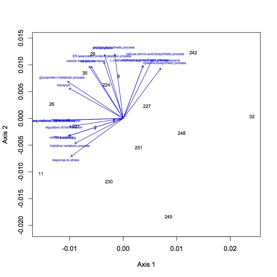
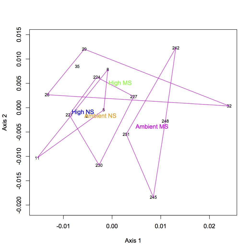
NMDS (GO) with polygons depicting treatment groups: https://www.evernote.com/shard/s242/sh/151d9a4b-59bc-4876-b071-e16838d23710/159fcaedd890a23decbc80f761be316c
http://eagle.fish.washington.edu/oyster/GO%20NMDS%20with%20polygons.pdf
ANOSIM indicated that the effect of pCO2 was significant on the differences among groups (p=0.029), there was no significant effect of just mechanical stress (MS), but there was a significant difference among groups when both stressors were considered (p=0.05).
ANOSIM of pCO2 effect only: https://www.evernote.com/shard/s242/sh/d7708eef-cdde-4b06-9f71-2e077dc7c808/135b60942113a8565a32d5eb53c92b99
http://eagle.fish.washington.edu/oyster/GO%20ANOSIM%20pCO2%20only.pdf
ANOSIM of pCO2 + MS: https://www.evernote.com/shard/s242/sh/75e585e6-5de2-4467-b701-63bfbd295506/45931721da1dfa657f5b7eea5614102f
http://eagle.fish.washington.edu/oyster/GO%20ANOSIM%20pCO2%20and%20MS.pdf
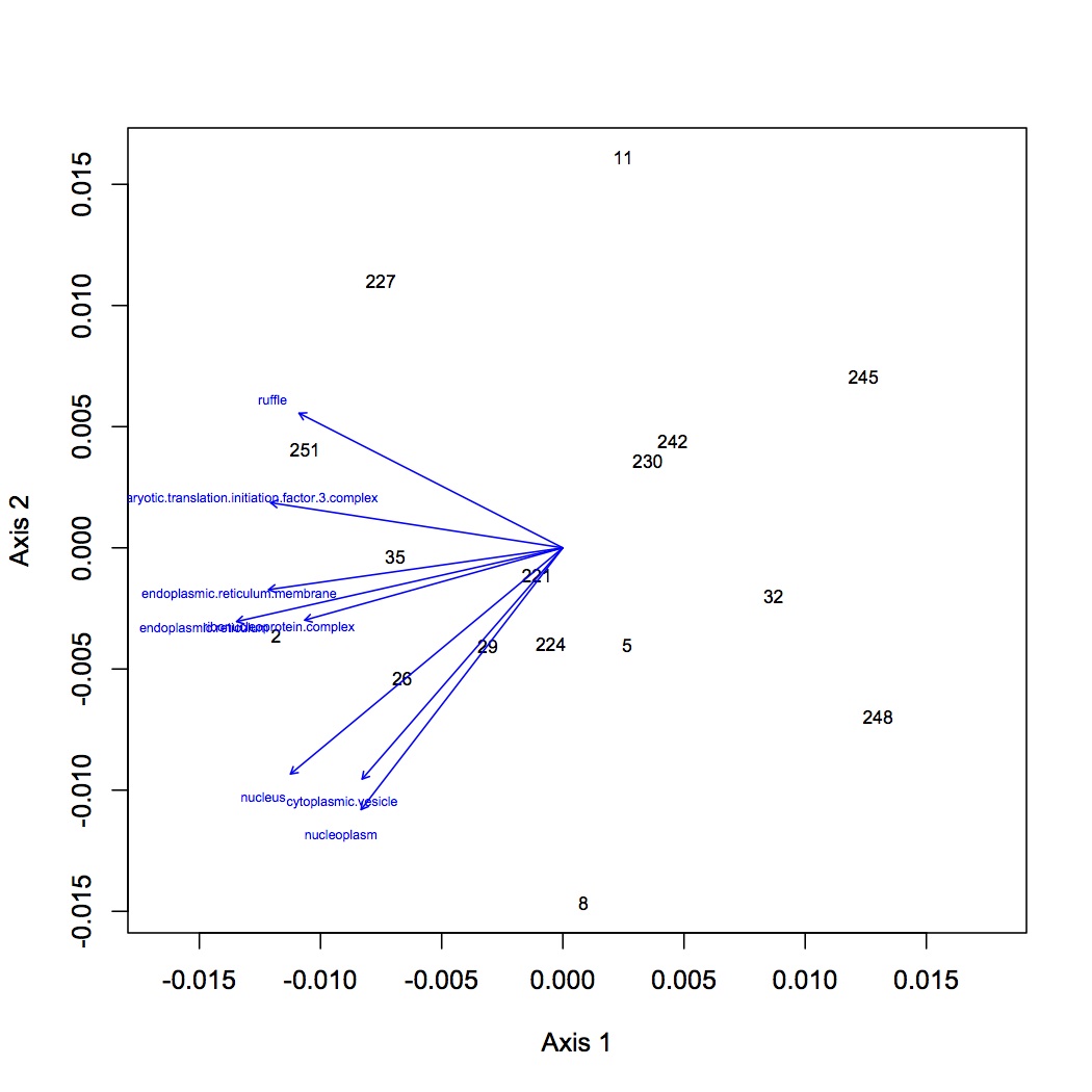
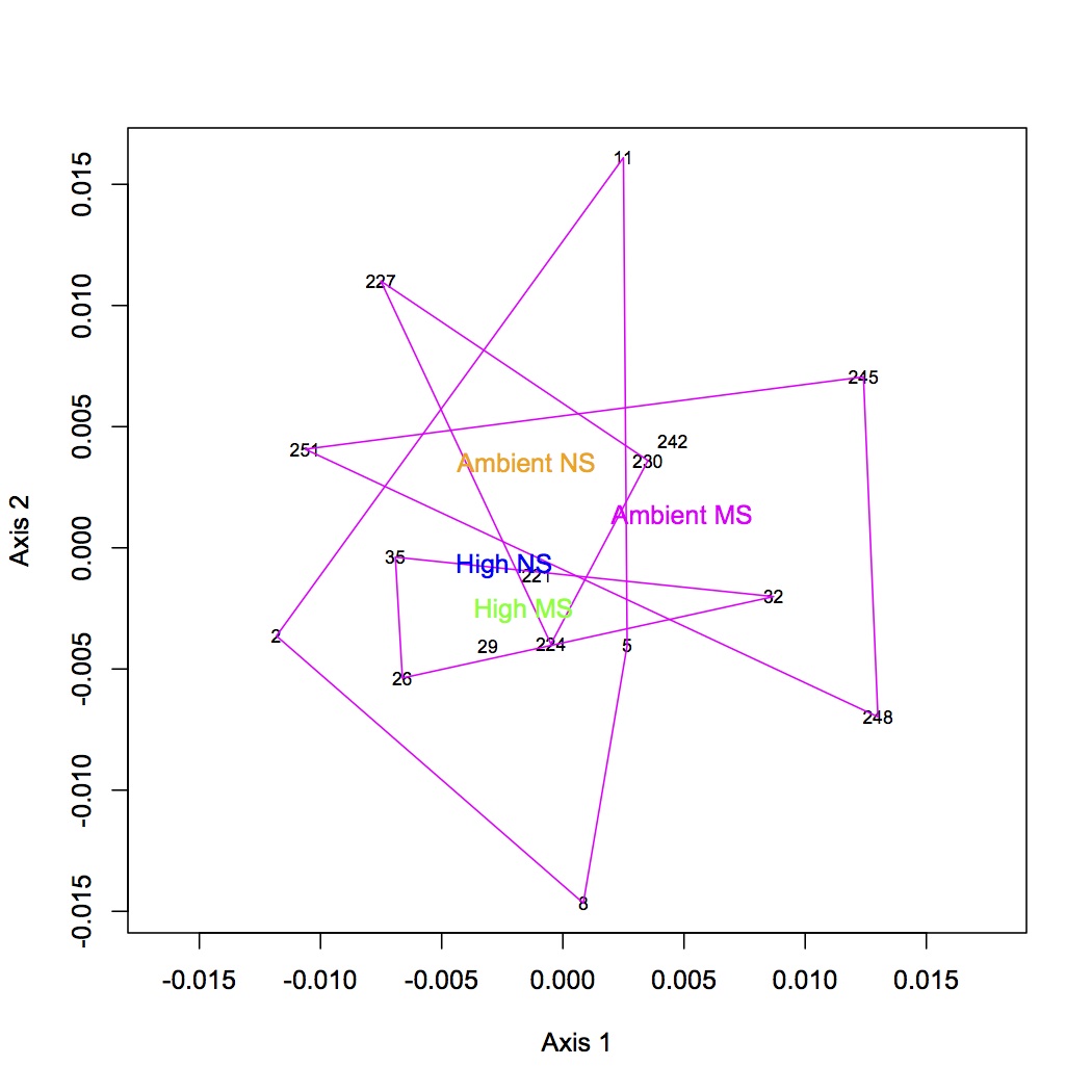
There are 98 individual GO terms corresponding to cellular components used in the multivariate analysis. After ANOSIM, there is no significant difference in protein express (for cellular components) among treatment groups.
NMDS with GO term loadings: https://www.evernote.com/shard/s242/sh/15800bfb-bd93-434d-815d-4b04ffb04f7b/f96eba07f7a7b54e18b803b4d711f94f
http://eagle.fish.washington.edu/oyster/GO%20components%20NMDS%20with%20loadings.pdf
NMDS with polygons: https://www.evernote.com/shard/s242/sh/8eaffd1c-f368-4d9d-985b-29f9e39f6736/9b62e0d175f214144db4135a4111541a
http://eagle.fish.washington.edu/oyster/GO%20components%20NMDS%20with%20polygons.pdf
December 7, 2012
Secondary Stress: Proteomics
Multivariate statistics for proteomics (based on a conversation with Julian Olden).
First round of analyses is on proteomics at the individual protein level. The input file is total spectral counts (across 3 technical replicates) for each biological replicate. I did the exact same NMDS for 4 different versions of the dataset: all proteins included, removed proteins that were low abundance (only expressed in 8 or fewer oyster, n=35 proteins), removed proteins that were high abundance (expressed in at least 95% of the oysters, n=779 proteins), removed both low and high abundance proteins. Each dataset was log-transformed and the Bray-Curtis dissimilarity coefficient was used. Only 2 dimensions were needed to explain the data. Links to the NMDS plots are below. The numbers represent individual oysters. 2-11 = high pCO2, 26-35 = high pCO2+mechanical stres, 221-230=ambient pCO2, 242-251 = ambient pCO2 + mechanical stress.
NMDS of dataset with low and high abundance proteins removed: https://www.evernote.com/shard/s242/sh/09f65203-1bde-4424-84a6-635083432b56/89538a8722f62427372be61c9cceccff
http://eagle.fish.washington.edu/oyster/NMDS%20no%20low%20high%20abundance%20120712.pdf
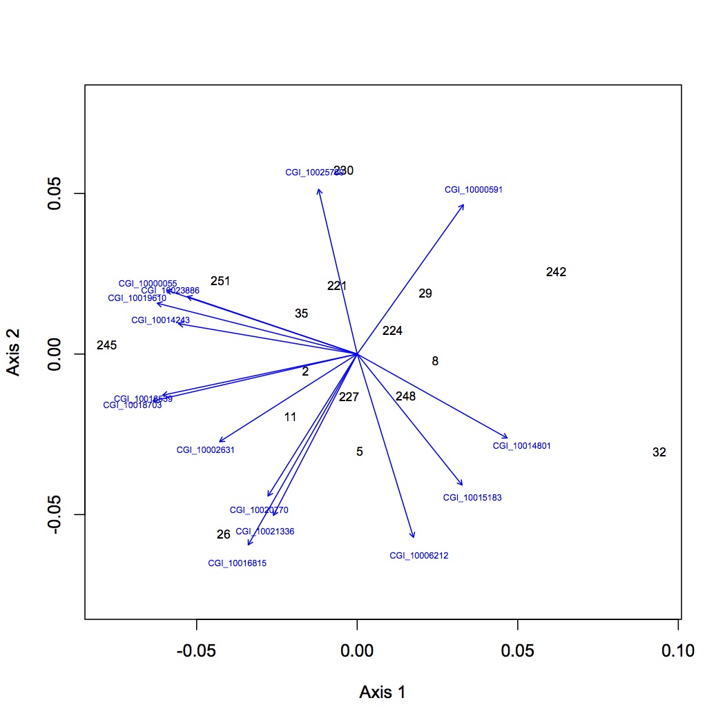
low abundance removed: https://www.evernote.com/shard/s242/sh/cae42bdb-14a9-4e1a-8fa4-e1475a8f1fad/bd876271d6ad157e9380ef200f9f9606
http://eagle.fish.washington.edu/oyster/NMDS%20no%20low%20abundance%20120712.pdf
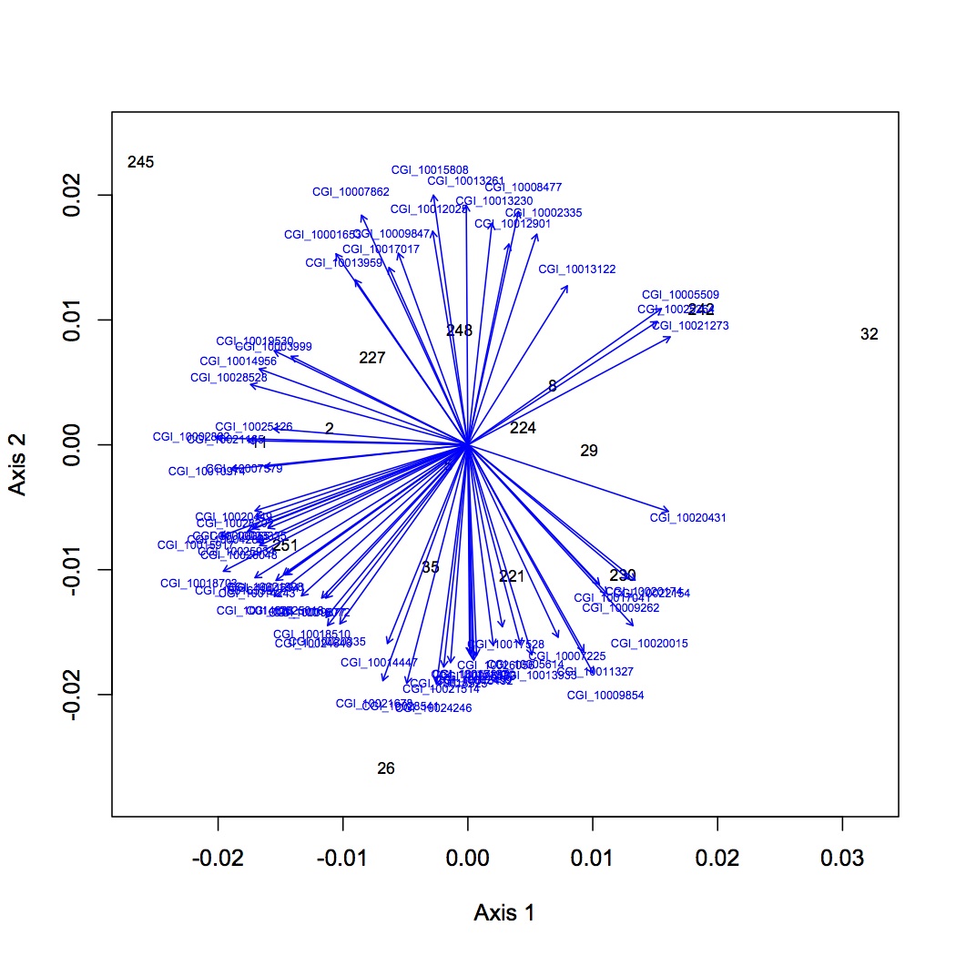
high abundance removed: https://www.evernote.com/shard/s242/sh/b32c814b-4041-47d9-a7ee-d26622fd26dd/0ac4a5868af643dedcf73183e19cf037
http://eagle.fish.washington.edu/oyster/NMDS%20no%20high%20abundance%20120712.pdf
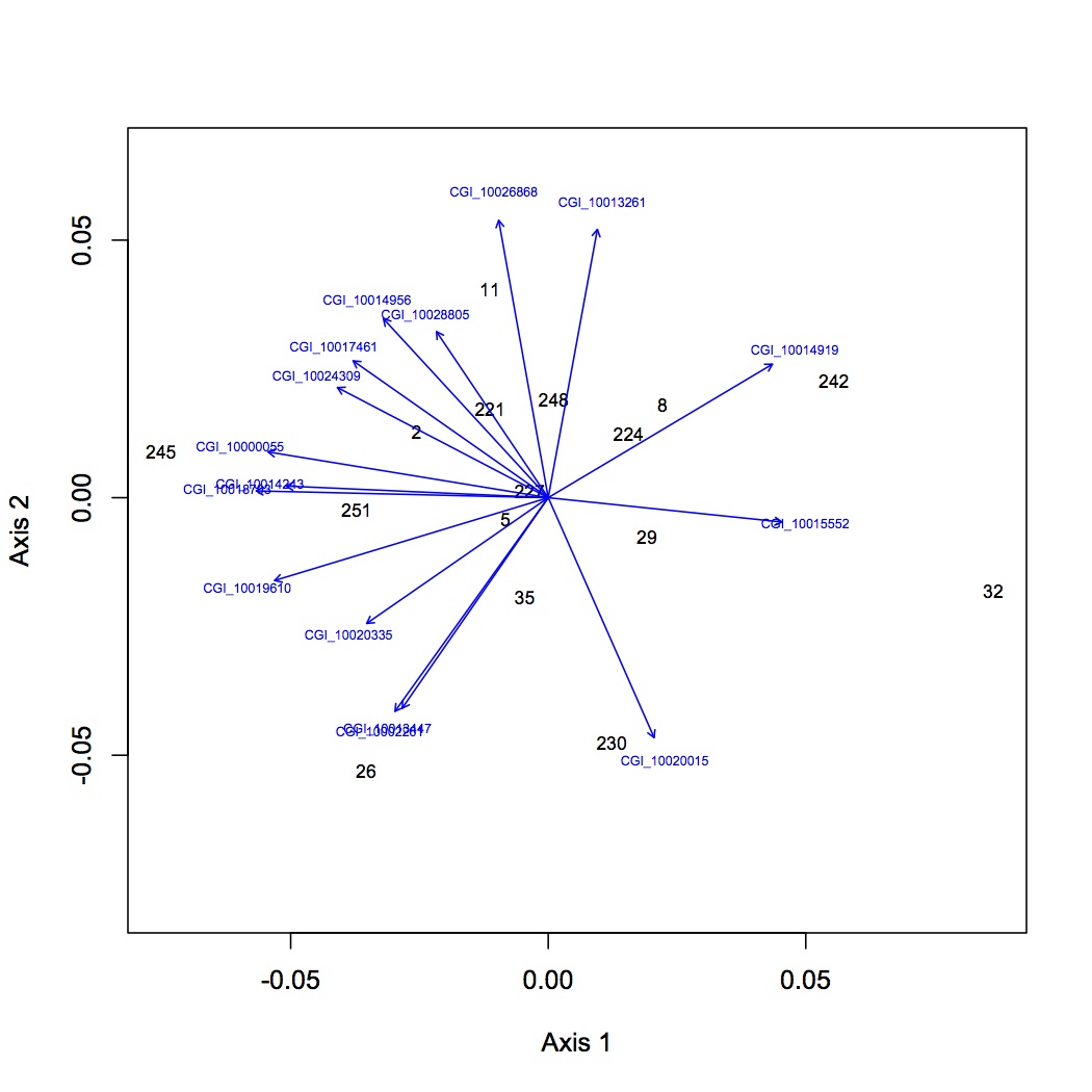
all proteins: https://www.evernote.com/shard/s242/sh/08eb3fe4-2465-488b-963b-adc9452f25de/c7f19a811b3f42fe8b6ffc6623206731
http://eagle.fish.washington.edu/oyster/NMDS%20all%20proteins%20120712.pdf
To determine which proteins are responsible for differences between oysters, joined all loading files together in Galaxy and annotated with SPIDs (no e-value cut-off). Annotated the NMDS's with protein identifications.
low and high abundance proteins removed: https://www.evernote.com/shard/s242/sh/f81ddfcd-d2fe-4ff4-8345-a61714202594/d7ed7ff37656bff529fa77abdacd965f
low abundance removed: https://www.evernote.com/shard/s242/sh/2a7af91c-9d73-4fe7-879a-22455f3e153c/a133015ab58a4c1894c485a8b439b710
high abundance removed: https://www.evernote.com/shard/s242/sh/5fcb81d6-8923-438e-9c76-3443aa74e659/a60e2f35c117063a2a12e8b88f4eebcb
all proteins: https://www.evernote.com/shard/s242/sh/f8b47757-8074-4c65-b547-cd7d513e861e/c60ba15924730a79f9dff7a2d6576e2c
In the NMDSs for all proteins and only low abundance proteins removed, there is quite a bit of redundancy in the proteins that explain the object (oyster) distribution in space. Even with the simpler plots, however, there does not seem to be a very clear pattern emerging.
December 6, 2012
Secondary Stress: Proteomics
Joined all protein prophet files together and then summed across technical replicates so that each biological replicated is represented by one column. Kept only the proteins that had at least 10 spectral counts across biological replicates. Did 2-tailed, type 2 t-tests in excel to identify proteins of interest for the following treatment groups: effect of mechanical stress in high pCO2 only, effect of mechanical stress in ambient only, effect of mechanical stress over both pCO2 groups, effect of pCO2 over all 16 oysters. Annotated the proteins with SPIDs and descriptions in Galaxy.
70 proteins were differentially expressed in the oysters exposed to mechanical stress (MS) at high pCO2. Some potential proteins of interest include hsp90, hsp70, multidrug resistance protein.
60 proteins were differentially expressed in the oysters exposed to MS at ambient pCO2. Some of these were the same as those differentially expressed at high pCO2, but they were the minority. Some differentially expressed proteins were Toll-interacting protein, cytochrome c oxidase, hsp70
67 proteins were differentially expressed in response to MS across pCO2 treatments. Most of these were differentially expressed in at least one pCO2 treatment.
67 proteins were differentially expressed in response to pCO2 and most of these were not differentially expressed in response to MS. These proteins included stress-induced phosphoprotein 1, v-type proton ATPase, hsp105, cathepsin L.
These combine results produce 219 unique proteins that are differentially expressed due to either pCO2, mechanical stress, or a combination. These 219 proteins will be used to create a protein and peptide tree in Skyline. I will also add proteins to the list from the statistics done yesterday on ambient vs. high pCO2 for a total of 357 proteins.
Downloaded the fasta file of the v9 proteome (local) from crassostreome and uploaded into Geneious. Manually made individual sequence documents for the proteins of interest to export as a single fasta file (C. gigas proteins for Skyline.fasta).
December 5, 2012
Secondary Stress: RNA-Seq
The output file from yesterday is uninformative because there are spaces in the contig names so for each query name it only picked up the first word (Consensus). Reformatted the file so that contig names are Contig1, Contig2, etc. and reran the blastn on the Mac mini with the output file called blastn_isotigs_120512.
Secondary Stress: Proteomics
To compare the effects of elevated pCO2 on the proteome, uploaded all replicates to Galaxy for just high pCO2 (no mechanical stress, samples Exp2.2, 5, 8, 11) and samples for just ambient pCO2 (221, 224, 227, 230). Within each treatment group, joined replicates based on protein identification number. (High pCO2 files were accidentally uploaded into the wrong workflow - C. gigas 3' RNA-Seq.)
Edited the Galaxy files so that they were just columns for total spectral counts for each replicate. Uploaded these files back into Galaxy and joined the 2 pCO2 treatments. Created a file so that each biological replicate (n=8) had just one column which contained the sum of total spectral counts for each protein. Analyzed this data in DESeq just to see what would happen. 56 proteins were "differentially expressed" according to DESeq, all of them downregulated (actually not expressed) at high pCO2 except for 1 protein. Annotated these proteins with SPIDs in Galaxy. Among the proteins down-regulated at high pCO2 were carbonic anhydrase (important for calcification), hsp70, complement component 1Q (immune response), cytochrome c oxidase, dual oxidase (regulated production of ROS).
Did a t-test of the summed total spectral counts to compare expression between the 2 pCO2 treatments (2-tailed, type 2 in Excel). 268 proteins showed differential expression using this method. Annotated the proteins in Galaxy. Removed proteins that had <10 spectral counts across the 8 replicates. This left 168 proteins with a significant t-test p value (<0.05). Most of the same proteins identified by DESeq were shown to be differentially expressed by the t-test method as well, except carbonic anhydrase was just over the threshold of non-significance (p=0.057). Other proteins that were not identified with DESeq were v-type proton ATPase, Toll-interacting protein, uncharacterized oxidoreductase, MAP kinase-activated protein kinase 2, stress-induced phosphoprotein.
December 4, 2012
Secondary Stress: RNA-Seq
Less than 50% of the reads mapped back to the consensus isotigs for each sample (EM2A-EM2H). Of the reads that mapped back, the large majority for each sample mapped uniquely to one isotig.
Exported all 8 RNA-Seq files as csv and resaved them as tab-delimited text files with names e.g. EM2A isotig RNA-Seq.txt. Uploaded to Galaxy. Joined all RNA-Seq files together based on contig number to make file "all isotig RNA-Seq joined". Exported to excel. Removed all isotigs that had less than 10 total reads mapped across all 8 samples - this is the file for DESeq (isotig RNA-Seq for deseq.csv).
Isotig 100818 is differentially expressed.
There is definitely redundancy in the isotigs (i.e. some of them map to the same transcript). I need to remove this redundancy by combining isotigs that map to the same transcript and redo the DESeq.
Exported the consensus sequences from the de novo assembly (the isotigs). Uploaded the fastq file to Galaxy and made it into a fasta file. Saved fasta file to Eagle so that it is accessible from the Mac mini when Eagle is mounted as a server. Created database of Sigenae v8 on the Mac mini by using the following in the Terminal (in the directory ncbi-blast-2.2.27+ in subfolder bin). Downloaded sigenae v8 transcriptome from crassostreome and made it into a database using makeblastdb. Ran blastn using the following code to blast the isotig consensus sequences against the sigenae db with a evalue cut-off of 1E-5, only the top hit returned.
./blastn -num_threads 8 -out [output file directory and name] -db [db directory and name] -outfmt 6 -evalue 1E-5 -max_target_seqs 1 -query [directory and name for isotig contigs] -task blastn
Output file is on Eagle (http://eagle.fish.washington.edu/oyster/blastn_isotigs_120412).
Secondary Stress: Proteomics
Edited all of the Protein Prophet output files so that they can be uploaded into Galaxy.
December 3, 2012
Secondary Stress: Proteomics
I have been uploading raw files into Skyline for analysis. Files were uploading without a problem until I tried to upload 101B_35 (see 11/30/12). I tried a few other files and get the same error. to make sure that it is a Skyline problem and not a file corruption problem, I created a new Skyline session called "test", uploaded one xml file as the library, and imported the 101B_35_01 as a results file. The file uploaded successfully, so there is a problem with Skyline.
Confirmed that the problem is not enough memory in the computer. With more memory I should be able to upload more files. There's also a possibility of partitioning the number of transitions and creating different documents for the different partitions (I'm not really sure what this means or what it would do to my analysis).
Secondary Stress: RNA-Seq
SR has done some work with the 3'-targeted data (see his notebook, Cgigas tag-seq). The idea is to do a de novo assembly to create isotigs and then map the isotigs to the transcriptome using strict parameters.
In CLC, did a de novo assembly of the reads trimmed for quality and virus sequence. Mismatch cost = 2, insertion cost = 3, deletion cost = 3, length fraction = 0.8, similarity = 0.95, vote conflict resolution, ignore non-specific matches, minimum contig length = 75. Saved in folder 'de novo 120312'.
of the 9,283,995 reads, 3,741,778 assembled into contigs with an average length of 95.25 (356,400,475 bases). The total number of contigs assembled = 115,999 with an average length of 126. The number of reads making up the isotigs ranged from 2-1,222,730 (this last is contig 61969). Selected all contigs and "open consensus" to create consensus sequences of the isotigs (saved in the same folder).
Mapped the extracted consensus isotigs to the Sigenae v8 transcriptome. Mismatch cost = 2, insertion cost = 3, deletion cost = 3, length fraction = 0.5, similarity = 0.95, vote conflict resolution, ignore non-specific matches.
Did the same mapping to reference except changed the similarity to 1 and to 0.8. Also mapped to the genome v9 (0.95 similarity).
Sigenae mapping, similarity = 0.95: Out of 115,999 isotigs, 42,647 mapped to Sigenae transcriptome with an average length of 129.64 (26,290 references). Again, it looks like the isotigs mapped all across gene sequences (i.e. they did not fall just at the 3' end). The number of isotigs mapping to a gene ranged from 1-22.
Sigenae mapping, similarity = 0.8: Out of 115,999 contigs, 47,976 mapped to the transcriptome with an average length of 129 (27,971 references). The number of isotigs mapping to a gene ranged from 1-34. Some isotigs mapped just on one end of a transcript (ES789949, DW713967), but many transcripts had isotigs mapping to multiple areas.
Sigenae mapping, similarity = 1: 28,889 isotigs mapped to the transcriptome with an average length of 128.41 (19,466 references). The number of isotigs mapping to a gene ranged from 1-21. Again, it looks like most transcripts had isotigs mapping to multiple areas, not just the 3' end.
genome mapping, similarity = 0.95: 74,149 isotigs mapped to the genome with an average length of 125.53 (1,657 references).
Preparing data to do DESeq. Did RNA-Seq on all the trimmed files, mapping back to the consensus sequences from the de novo assembly. max number of mismatches = 2, min length fraction = 0.9, max number of hits for a read = 10, expression value = RPKM. Saved outputs in RNA Seq folder under de novo 120312.
November 30, 2012
Secondary Stress: Proteomics
Trying to decrease the amount of time and memory it takes to import raw files into Skyline.
Settings > Transition settings > full scan > retention time filtering: use only scans within 5 minutes of MS/MS IDs.. This should significantly reduce the amount of time/memory it takes to import raw files.
This change has significantly reduced the memory the computer uses to import raw files. I will need to go back and change 101B_11 and 101B_32, which were imported without the chromatogram limits.
When I tried to import the file 101B_35_01, I got an error message: Failed to build a cache for "...Sklyine 112812.sky.", Failed to create cache "...Skyline 112812.skyd." Skyline ran out of memory.
From looking at the online help forum, it seems that this message means that there is something wrong with the actual data file.
November 28, 2012
Secondary Stress: Proteomics
Created new library of pepXML files using the v9 interact files (these are filtered for high probability of peptide identification). The library is called "interact" and is made up of all biological and technical replicates. Made changes in peptide settings and transition settings as previously described. In Spectral library explorer, added all peptides to the peptide tree and included the peptides that did not match the filter settings. There are 25,710 peptides total. Saved the Skyline session as Skyline 112812.
Imported raw data files. File > Import > Results > Add single-injection replicates in files > 101B_11_01.
Settings > check Integrate all
Changed peak areas settings as described 11/26/12.
Imported other 2 technical replicates as additional replicates for 101B_11_01.
November 26, 2012
Secondary Stress: Proteomics
Analysis of protein expression in Skyline.
Created spectral library in Sklyline using xml file from 101B_2_01 as described 11/21/12. File used was in the v9 subfolder of 20120821_OT1.
Repeated the same steps to add the spectral library for 101B_2_02 except used the file from the 20120821_OT1 folder (I wanted to see if either spectral library would include annotations for protein IDs, neither did so I deleted this library). Created spectral libraries for 101B_2_02 and 101B_2_03 using the v9 XML file.
Made library for 101B_5 by adding files for all 3 technical replicates. This seemed to work, so created a library called Cg Gill and added all pepXML files to it from v9 folder. This resulted in 0 spectra being found to put in the library. Made a library called 101B with all of the pepXML files from high pCO2 oysters. This library has over 112,000 spectra in it. Saved the Skyline document as Skyline 112612.
File > Import > Results > Add one new replicate: Name 101B_2_01, optimizing none.
Settings: Selected (to check) "integrate all"
View > peak areas > Replicate comparison: right click in window and make sure under Normalize to "none" is checked and Show expected and Show dot products are checked.
File > Import > Results > Add files to existing replicate: 101B_2_01, selected raw file for 101B_2_02. Repeated for 3rd technical replicate.
Emailed with Jimmy and the v9 subfolder contains SEQUEST results from searching the spectra against the genome database. The pepXML files not in that subfolder are from searches against the translated Sigenae database. From here on out, only pepXML files in the v9 subfolder will be used for analyses.
November 21, 2012
Secondary Stress: Proteomics
Analysis of protein expression in Skyline.
Settings > Peptide settings > Digestion: enzyme = trypsin [KR/P], max missed cleavages = 2, background proteome = none.
Peptide settings > Modifications: Carbamidomethyl cysteine and Oxidation (M). Check Variable box.
Peptide settings > Library > Build: name = 101B_11_01, check Keep redundant library, cut-off score = 0.95, lab authority = roberts.fish.washington.edu. Next > Add files: Add the orbitrap mzXML file.
Peptide settings > Library: check 101B_11_01, Pick peptides matching = Library.
individual libraries for each replicate need to be built one at a time.
Settings > Transition settings > Filter: Precursor charges = 2,3,4, Ion charges = 1,2,3, ion types = p, check auto select all matching transitions.
Transition settings > Library: uncheck if a library spectrum is available pick its most intense ions.
Transition settings > Full-scan: isotope peaks included = count, precursor mass analyzer = orbitrap, peaks = 3, resolving power = 60,000 at 400
In spectral library explorer, clicked Add all to add all peptides (357 peptides did not match the current filter settings, chose to include them).
Repeated above steps for 101B_11_02 library.
November 20, 2012**
Secondary Stress: RNA-Seq
Ran experiment in clc on the RNA-Seq (transcriptome) to compare expression between the 2 pCO2 levels. Filtered the data so that only genes remained that showed at least 2-fold difference between the two treatments (~24,000 genes, compared to original 82,000). Exported this file as a .csv. Added column to file that compares expression values using a t-test. Uploaded file to Galaxy and joined with gene annotations of the Sigenae IDs, GO, and GO Slim. Looked through genes that had a p-value (from t test) of less than 0.05 and highlighted genes of interest in yellow. These genes are listed below with an "x" in the column for the treatment in which they are more highly expressed.
| Gene |
400 µatm |
2800 µatm |
| fibroleukin |
x |
|
| apoptosis inhibitor 5 |
x |
|
| calcitonin receptor |
x |
|
| v-type proton ATPase |
x |
|
| MAPK |
x |
|
| big defensin |
x |
|
| acid ceramidase |
x |
November 19, 2012
Secondary Stress: RNA-Seq
Will try DESeq on the reads mapped to the genome (DESeq done 11/16 was on reads mapped to the transcriptome). For each library (EM2A-EM2H), did RNA-Seq on the clc server, mapping to the genome v9. Minimum length fraction = 0.9, max number of hits for a read = 10, expression value = RPKM. Saved in folder RNA-Seq for trimmed reads (genome).
Exported RNA-Seq files as .csv and uploaded into local Galaxy online. Joined all files together based on scaffold number. Created an input file for DESeq with 1 column for the total reads in each library. Deleted rows that had total reads summing across libraries to <10. (I realize that it doesn't completely make sense to be doing differential expression based on scaffolds because each scaffold represents multiple genes, but I figure that it's a starting point and if I see differences at the scaffold level I can try to bring it down to the gene level.) the file is called "oyster genome for deseq.csv". Output is saved as "C. gigas OA Result Table genome RNA-Seq.csv". None of the scaffolds are significantly differentially expressed, but 4 have an adjusted p-value <1 (and significant p-value): scaffolds 1590, 39732, 42598, and 521.
Figures:
Variance dispersion:
https://www.evernote.com/shard/s242/sh/9215445c-443c-442d-b28b-27acc8a95dfc/8f83c898b2ac54c9fdc9523e3cff8346
Significantly differentially expressed genes would be in red on this plot:
https://www.evernote.com/shard/s242/sh/8e4a611c-0aeb-41ee-9f90-d6ac3e9018b5/868751f74998b939dac886d225afa258
p-value distribution:
https://www.evernote.com/shard/s242/sh/38d2bd7e-1257-40bd-b654-f594c94af1d9/c607524f12aff0960902cbb1bfff899f
November 16, 2012
Secondary Stress: RNA-Seq
Downloaded genes file from oyster genome via crassostreome (local version, oyster_v9_gene.fasta). Mapped reads (quality and virus trimmed) from individual oysters to the gene file using Map reads to reference on server. mismatch cost = 2, insertion cost = 3, deletion cost = 3, length fraction = 0.5, similarity = 0.8, no global alignment, vote conflict resolution, ignore non-specific matches. Mappings saved in Gene Mapping folder.
There were many fewer read matches in the mapping of reads to gene sequences. For example, in sample EM2A out of 1,409,302 reads 106,515 matched when the reads were mapped to genes, 508,285 mapped to the Sigenae transcriptome, and 982,720 mapped to the genome scaffolds.
Redid DESeq with contigs that had at least 10 reads across all 8 samples (n=13,111). The adjusted p-value was still = 1 for all comparisons of differential expression between treatments. See figures from analysis below.
Variance dispersion: https://www.evernote.com/shard/s242/sh/747a7ef2-03b2-4626-b24f-13369f98f8ec/05191a88ee0b205d62770cb878985c9a
Significantly differentially expressed genes would be in red on this plot: https://www.evernote.com/shard/s242/sh/7c34fac2-0e7b-47c5-9349-11d95dbb5064/9968f10465028367bdef30eb26c56c71
p-value distribution: https://www.evernote.com/shard/s242/sh/0ec4cca3-83e5-4116-8a37-0dcd2ebfa514/2275e5c6dc12de5d483b510a6b8d95db
November 15, 2012
Secondary Stress: RNA-Seq
Comparison of expression between treatment groups in clc. Created consensus sequences for all reads mapped to Sigenae v8 by opening the mapped reads, selecting all sequences, and clicking "open consensus". For each consensus sequences did RNA-Seq on the server. Used cgigas_all_contigs_v8 as the reference without annotation. Assembly settings: Max # mismatches = 2, min length fraction = 0.9, max # hits for a read = 10. Expression value set at RPKM. These RNS-Seq files are saved in subfolder under "sigenae mapping" called "RNA-Seq analysis (consensus seqs)".
Did RNA-Seq for the trimmed reads (quality and for virus). Same parameters as above. Results saved in folder "RNA-Seq for trimmed reads". Exported these files as tab-delimited text.
DESeq wasn't loading because I needed to update my R package. R was updated and I was able to load DESeq. Following the user manual (http://bioconductor.org/packages/devel/bioc/vignettes/DESeq/inst/doc/DESeq.pdf), I am putting together an input file and starting my analysis with the files created from the RNA-Seq of the trimmed reads (see above). The expression values in the input file need to be raw counts of sequence reads (total reads in clc terminology). The rows of the file should be individual transcripts and each column should be the expression values for a sample. Made this file in Galaxy by joining all of the RNA-Seq files together. Removed all rows that had 0 expression across all samples, formatted cells as "general" (otherwise R does not recognize cell contents as numbers), and saved as csv file "oyster for deseq".
November 14, 2012
Secondary Stress: RNA-Seq
Added sequence for virus PhiX174 as adapter to be trimmed since it is possibly part of the sequence information. Eli sent a file with its genome sequence. In clc: Edit > Preferences > Data. At the bottom of the adapter trimming table, click "Add row". Adapter is called Illumina phiX, entered entire genome as sequence, strand=plus, alignment score = 2,3,10,4, action= remove adapter. Eli also said that "GGG" or "GGGG" may be present at the 5' end of some of the sequences, but I'm not sure how to tell clc to only trim "G" repeats at the 5' end and Eli said it shouldn't be a problem. Saved these trimmed reads in the folder PhiX trimmed. ~100% of the original reads were still present after trimming, meaning that there was not much virus sequence in the reads.
Downloaded cgigas_all_contigs_v8.fa to use as reference for assembly of trimmed reads (Sigenae transcriptome). Mapped the doubly trimmed reads to the transcriptome (individually) and saved in Sigenae mapping folder: mismatch cost = 2, insertion cost = 3, deletion cost = 3, length fraction = 0.5, similarity = 0.8, no global alignment, vote conflict resolution, ignore non-specific matches.
Exported mapping file (.sam) for EM2B to Eagle. Uploaded to local Galaxy on the web and named EM2B Sigenae. Visualized in Trackster using Sigenae contigs v8. There was an error in visualization, so redid the same steps on the public Galaxy website.
Exploring IGV: downloaded IGV from website. Loaded C. gigas Sigenae v8 as a "genome" in IGV by selecting Load genome from URL from the File menu. Downloaded EM2B file mapped to Sigenae and created index file in igv: File > run igvtools, command = index, browse for file and hit run. Index file is saved in same folder as .sam file. Loaded .sam file into IGV by going File > Load File. Contigs can be viewed individually with mapped reads. The multicolored bar at the bottom of the screen is the contig sequence, the gray bars are the mapped reads. The colors in the gray bars are SNPs between the reads and the contig.
See IGV view here:
https://www.evernote.com/shard/s242/sh/05aa2bb4-441b-4655-9976-3e479c98fb91/0076c89fc20d887a4b05fc94f11e106c
Decided to go ahead and try to do RNA-Seq to see what happens. I would like to try this in the R package DESeq. I tried to install DESeq but it seems that the website is currently down (I found on a discussion board that this is likely to happen). I'll try to install it again tomorrow.
November 13, 2012
Secondary Stress: RNA-Seq
The local Galaxy mapping started on the Mac mini on Nov 7 is still running.
Downloaded and unzipped files on the PC in the lab to start workflow in clc. Logged into clc server and created directory: C. gigas OA RNA-Seq. Imported sequence files (EM2A-EM2H) into this directory by importing high throughput sequencing files and choosing Illumina as the data type. Also imported oyster.v9_90 genome file to use as reference (this was imported just through the normal file import).
Mapped EM2A to oyster genome v9. Parameters were: mismatch cost =2, insertion cost = 3, deletion cost = 3, length fraction = 0.5, similarity = 0.8, no global alignment, vote conflict resolution, random non-specific matches. Saved mapping in sub-folder EM2A (this mapping was done locally). Queued EM2B-EM2H to map to the reference with the same parameters but on the server.
Exported mapped reads at .sam files and uploaded to Galaxy. In Galaxy, .sam files can be converted to interval files and then to BED files. (We discovered that sam files have the same depth info as bed files so the conversion may not be necessary.) Both sam and bed files can be visualized in Trackster (saved visualization as EM2A SAM1). Saved oyster.v9_90 as a reference genome in Galaxy. Viewed sam and bed files with genome as reference. Added oyster v9 annotations for CDS (exons) and mRNA (gene sequence, probably does not include UTR) as tracks in the visualization. A lot of the reads seem to fall into improbably areas on the gene. We will try mapping cleaner reads to the transcriptome (from Sigenae).
Example of visualization:
https://www.evernote.com/shard/s242/sh/e5261617-2ed7-43c9-a7a7-79e72db5d705/0a8e9fc59b201a0a8f26bc5ddd60c6ef
Quality trimmed the reads in clc: trim using quality scores, limit = 0.05, trim ambiguos nucleotides, maximum number of ambiguities = 2, discard reads less than 50. About 70-75% of the reads for each sample were retained after trimming (see below). Mapped these trimmed reads to the genome. Next steps: remove barcodes and other excess sequences.
Trim report:
https://www.evernote.com/shard/s242/sh/4bbfb2be-3afa-478a-aa89-fac20a77e145/5704e8d29c98a658396bd609fce14c6e
https://www.evernote.com/shard/s242/sh/eeb61897-f3c8-462e-9927-214170636888/9ade273133af8f8ab5db524995dae33d
November 7, 2012
Secondary Stress: RNA-Seq
Data from NGS run by Eli Meyer is on Eagle (http://eagle.fish.washington.edu/oyster/gigas_rnaseq.tar.gz). The sample IDs are explained in the table below. Began analysis of sequence data on local Galaxy on the Mac Mini. Created an admin account on the mini and opened terminal to launch Galaxy. In terminal, entered the following code:
cd /Users
cd Shared
cd Apps
cd galaxy-dist
./run/.sh
Opened a web browser and entered address: localhost:8080
Username for the local Galaxy is my gmail address.
Saved unzipped fastq files in Documents on Mac mini and also on my laptop. Uploaded the first file (EM2A.fastq) to Galaxy on the mini. This is taking a really long time, so decided to start running on Geneious on the mini.
Geneious:
Downloaded C. gigas genome from crassostreome (oyster.v9_90, fasta file) and uploaded into Geneious. Also uploaded EM2A. Mapped EM2A sequenced to genome reference. Sensitivity = medium-low sensitivity/fast, fine tuning = none (fast/read mapping), no trimming sequences, saved in sub-folder, and saved contigs...Oops, not enough memory to perform the assembly.
Local Galaxy:
Uploaded oyster.v9_90 to galaxy as well. Named history "C. gigas 3' RNA-Seq". Made oyster genome into a reference sequence: under "Visualization" at the top of the page, chose new visualization, and then clicked add a custom build. Named the reference "C. gigas genome v9". Uploaded other fastq data files into history. Under tool heading "NGS: QC & manipulation" used the FASTQ to FASTA converter to make all files FASTA.
Mapped EM2B to the reference genome using the NGS Mapping tool Lastz (for mapping short reads to a reference). Output = tabular, commonly used settings, mapping mode =Illumina 95% identity, ept min and max reporting and coverage reporting the same (0, 100, 0).
| Meyer ID |
BC # |
ETS ID |
pCO2 |
| EM2A |
BC1 |
Exp2.1 |
2800 |
| EM2B |
BC51 |
Exp2.4 |
2800 |
| 2C |
52 |
7 |
2800 |
| 2D |
53 |
10 |
2800 |
| 2E |
57 |
217 |
400 |
| 2F |
58 |
220 |
400 |
| 2G |
54 |
235 |
400 |
| 2H |
55 |
238 |
400 |
October 31, 2012
Bioinformatics: Pinto Ab NGS
Oly SRA files were successfully transferred the second time. The correct accession number for the Oly and Pinto RNA-Seq data is
SRA057107.
October 30, 2012
Proteomics: Analysis for Manuscript
Compared protein identifications across technical replicates. Created csv file tech reps for plotting which has a column for each technical replicates across all 4 biological replicates. Each cell with a number in it for a technical replicate means that protein was identified in that particular injection (proteins are listed in the far lefthand column). The matches across replicates were summed in the far righthand column and all columns were sorted based on number of matches. Graphed in R, color coding for biological rep (https://www.evernote.com/shard/s242/sh/47cb9fd2-873e-4ac9-a238-61220a48e04f/548adcdfa1cd42c0ca3963457e4062b9).
Plotted average spectral counts (proxy for protein expression) versus the number of times that protein was identified (or number of matches). The csv file is called spec counts tech reps (https://www.evernote.com/shard/s242/sh/092028b9-8e41-40fd-aeaa-701e31af3c77/324139ae3e2e0e5673fa76375a88590a). Did the same plot but using total spectral counts instead of average and got same result (not shown).
October 29, 2012
Proteomics: Analysis for Manuscript
These analyses were done only for the Orbitrap data.
Used Venny to create a Venn diagram comparing proteins expressed across biological replicates. From excel file ambient gill proteome joined to all replicates, got the list of protein IDs for expressed proteins for each oyster. For every protein that was expressed per oyster, copied the list into Venny.
Compared the 10 proteins that are expressed the most highly across biological replicates. From average spectral counts across technical replicates, determined which proteins were in the top 10 for each oyster. Protein annotations are provided by SPIDs. No oyster had a unique protein in this category. 8 proteins were included in the top 10 across all oysters.
Bioinformatics: Pinto Ab NGS
Got an email informing me that the Oly SRA files uploaded to NCBI were corrupted (original upload done August 10, 2012). Downloaded the fastq files again (
http://eagle.fish.washington.edu/whale/index.php?dir=&sort=date&order=desc). Files were renamed Olurida_R1 and Olurida_R2. In SRA submission, flow cell and lane numbers were kept the same (since it is the same data). Generated new checksums using MD5 software. Transferred files using FileZilla 2.
October 4, 2012
Secondary Stress: Fatty acids
Through conversations with Louise Copeman (NOAA, Newport, OR) and Michael Brett (UW) I've been learning a little bit about fatty acid analysis and what it can tell me about oysters and ocean acidification. Louise suggested that I investigate lipid class analysis as well as/instead of FA because it gives a good condition index (look at total lipid, storage vs. membrane lipids). She is set up to do this at OSU. If I did the extractions myself, lipid class analysis would be ~$80/sample and FAs would be $40/sample.
Michael Brett thinks that FAs can still give me some very useful and interesting information. FAs give insight into nutritional physiology and the quality of nutrition that an animal is getting. Lipid class tells you more the quantity of lipids being stored and which lipids are being stored. (During a FA analysis lipids are methylated so you don't know where they came from.) Lipid class analysis would should where the FAs end up and could answer the question: does OA affect the oyster's ability to withstand periods of low food? If I were to do FA with the Brett lab and do the work myself, it would cost $15/sample.
October 2, 2012
Bioinformatics: Pinto Ab NGS
Steven ran blast comparisons of both transcriptomes vs. Lottia gigantea proteins yesterday. In OrthoDB, got conserved proteins across all metazoans with a single copy in Lottia. SR did a tblastn of O. lurida and H. kamtschatkana contigs against this db of protein sequences (30 Lottia sequences total). O. lurida had 28 matches with an e-value less than 1E-5 and H. kamtschatkana had 2 matches.
For each contig that matched to a L. gigantea protein, translated in all 6 frames using standard sequence translation (Geneious). Aligned all 6 translations with the protein sequence: Geneious alignment, cost matrix = BLOSUM 6, gap open penalty = 12, gap extension penalty = 3, global alignment with free end gaps, 2 refinement iterations. From the alignment, determined the correct translation. Calculated the % of the protein that is covered by each sequenced contig.
Calculated # of SNPs per contig. SR had a table of all SNPs (http://aquacul4.fish.washington.edu/~steven/armina/OlyOSNPsAnnotated.txt and http://aquacul4.fish.washington.edu/~steven/armina/HkamSNPsAnnotated.txt). Downloaded table, put contig names in a column and made pivot table of column of contig names. Since each snp is a unique entry, a contig with multiple SNPs is entered multiple times. Took the average of the number of occurrences of/SNPs in each contig. for O. lurida this is 3.04, for H. kam this is 1.95.
October 1, 2012
Bioinformatics: Pinto Ab NGS
Computed contig lengths for assembles of Pinto and Oly transcriptomes to create histograms. Imported assembled contig FASTAs into Galaxy and used tool "compute sequence length" under FASTA manipulation. Kept all title characters. Exported contig length files (one column = contig name, second column = each contigs length) and made histograms in R.
Proteomics: Analysis for Manuscript
Uploaded protein prophet files to server for archiving. Server address is afp://128.95.149.204. Mount "web" to archive data. Created folder "oyster" and subfolder "proteomics" and copied all data into proteomics. Can be found here: http://128.95.149.204/oyster/index.php?dir=proteomics%2F
September 28, 2012
Proteomics: Analysis for manuscript
Did analysis of technical replicates to visualize variability with samples. For each oyster (103 B 221, 224, 227, 230), averaged the total number of independent spectra into a column called "average spectra". Created a csv file for R with protein name, total independent spectra for each technical replicate, and average spectra. Sorted all columns by average spectra, larges to smallest. Plotted each column of total independent spectra: replicate 1 = black, rep 2 = blue, rep 3 = green. Below is the plot for 103B230.
Bioinformatics
Downloaded new SwissProt associations database for annotations (SwissProt IDs linked with gene descriptions/annotations). Went to EMBL website and clicked on UniProtKB.
September 24, 2012
Proteomics: Analysis for manuscript
Downloaded proteome from the genome sequencing webpage. SR annotated the proteome with SwissProt IDs with an e-value cut off of 1E-10.
Jimmy re-ran SEQUEST searches of Orbitrap (OT) and QExactive (QE) data against the new database. downloaded all files with protein probability of at least 0.9. Further analysis is only on proteins from 103B 221, 224, 227, and 230 (ambient, not mechanical stress). All protein prophet files were annotated with SPIDS and joined to the proteome downloaded from the genome.
Made file of proteome for just the samples being analyzed (proteome 2). This is a list of unique contigs representing all the proteins sequenced in the triplicate injections of the 4 samples. Proteins are included only if they have at least 4 spectral counts across samples (1,672 proteins).
Using DAVID v. 6.7 did enrichment analysis of gill proteome sequenced vs. entire proteome downloaded.
Also did enrichment analysis of each oyster (across replicates) vs. proteome 2 to compare inter-individual variability. For all revigo files downloaded, they are the tables from the Gene Ontology BP FAT.
Visualized entire gill proteome by joining to GO terms, filtering out unique entries of contig-GO combinations, and putting in revigo. The number used in revigo was number of spectral counts across oysters/replicates.
